Numerical simulation of an extreme haze pollution event over the North China Plain based on initial and boundary condition ensembles

Figures & data

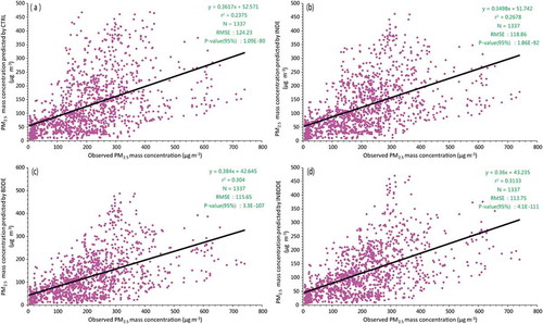
Figure 1. The model domain with elevation (shaded; units: m). Blue, purple, red, and black dots denote the observed hourly averaged PM_2.5 concentration (units: μg m⁻³) during 26 November to 2 December. The abbreviations BJ, TJ, BD, CZ, SJZ, HS, XT, and HD denote the eight cities as defined in the text.

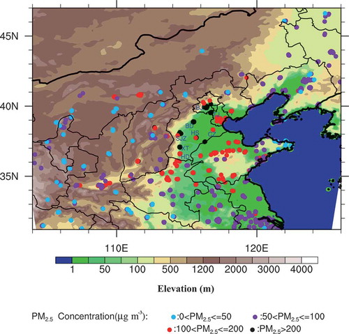
Table 1. Brief description of the initial conditions and LBCs in the CTRL, INDE, BDDE, and INBDDE experiments.

Experiment	Experiment description	Experiment members
CTRL	Model initial conditions and LBCs (updated hourly) were from HRES	1
INDE	Model initial conditions were from each of the 10 EDA members, and the LBCs were the same as in the CTRL run	10
BDDE	Model LBCs were from each of the 10 EDA members (updated every 3 h), and the initial conditions were the same as in the CTRL run	10
INBDDE	Both model initial conditions and LBCs (updated every 3 h) were from each of the 10 EDA members	10

Figure 2. (a) Hourly PM_2.5 concentration time series in eight cities predicted by CTRL (blue line), the INBDDE ensemble mean (red line), and the observation (black line). Pink filling represents the maximum and minimum range (or dispersion) of the forecasting results of 10 ensemble members. The correlation coefficients between the forecasting concentration of CTRL, INBDDE and the observed values are marked on the left-hand side. The bottom panel (b) is the same as (a), but for CO.

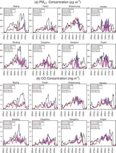
Figure 3. Scatterplots of the observed PM_2.5 concentration (units: μg m⁻³) in eight cities and the predicted PM_2.5 concentration from (a) CTRL, (b) INDE, (c) BDDE and (d) INBDDE, respectively. The black lines indicate the linear trend estimation based on the least-squares method.

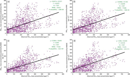
Table 2. Statistics of PM_2.5 concentration (units: μg m⁻³) and surface meteorological variables in CTRL, INDE, BDDE, and INBDDE. RH2M and T2M denote the relative humidity (units: %) and temperature (units: °C) at 2 m near the ground; WS10 and WD10 denote the wind speed (units: m s⁻¹) and direction (units: °) at 10 m near the ground. The ensemble mean values of the above variables were used to compute the statistical parameters in INDE, BDDE, and INBDDE.

Variable	Number of samples	Experiment	Bias	R	RMSE	EE
PM2.5 (μg m^−3)	1337	CTRL	−77.95	0.49	124.23	0
		INDE	−81.20	0.52	118.86	−4.33%
		BDDE	−83.32	0.55	115.65	−6.91%
		INBDDE	−87.63	0.56	113.75	−8.44%
RH2M (%)	1337	CTRL	−7.24	0.78	13.38	0
		INDE	−7.84	0.79	13.23	−1.10%
		BDDE	−6.85	0.78	13.47	0.70%
		INBDDE	−7.48	0.79	13.49	0.81%
T2M (°C)	1336	CTRL	0.26	0.83	2.04	0
		INDE	0.41	0.83	2.01	−1.20%
		BDDE	0.24	0.83	2.04	0.13%
		INBDDE	0.37	0.83	2.04	0.03%
WS10(m s^−1)	1336	CTRL	1.31	0.61	1.47	0
		INDE	1.32	0.62	1.46	−0.75%
		BDDE	1.29	0.64	1.48	0.56%
		INBDDE	1.30	0.64	1.50	2.32%
WD10 (°)	1336	CTRL	−16.84	0.26	133.29	0
		INDE	−18.89	0.27	126.37	−5.19%
		BDDE	−14.74	0.29	121.45	−8.89%
		INBDDE	−15.73	0.29	120.49	−9.61%

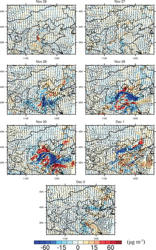
Figure 4. Differences of daily mean PM_2.5 concentration (shaded; units: μg m⁻³) and 10 m wind vector between the INBDDE ensemble mean and CTRL from 26 November to 2 December.