Energetics characteristics accounting for the low-level wind’s rapid enhancement associated with an extreme explosive extratropical cyclone over the western North Pacific Ocean

Figures & data

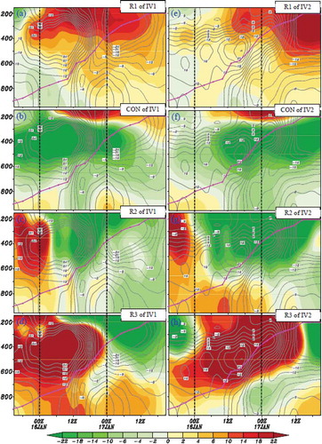
Figure 1. The left-hand column shows the 900-hPa total wind KE (shading; units: J kg⁻¹) and nonorthogonal wind KE (black lines with an interval of 20 J kg⁻¹). The right-hand column shows the 900-hPa rotational wind KE (shading; units: J kg⁻¹) and divergent wind KE (black lines with an interval of 10 J kg⁻¹). The red solid box shows the central region (12° × 12°) of Cyclone A, and the purple dashed boxes illustrate 16 key regions (6° × 6°) of the cyclone.

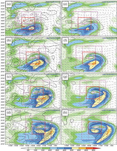
Figure 2. Total region (a) and each key region (b–q) averaged rotational (shading; units: J kg⁻¹) and divergent wind KE (black solid lines with an interval of 2 J kg⁻¹), where the solid purple line marks the top level of the cyclone and the gray-dashed lines show the maximum development stage.

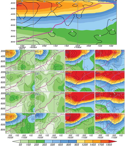
Figure 3. Budget terms of the rotational wind KE (shading; units: 10⁻³ J kg⁻¹s⁻¹) averaged within IV1 and IV2 (purple dashed boxes shown in Figure 1(a)), where the gray contours are TOT_R (units: 10⁻³ J kg⁻¹s⁻¹, with an interval of 3 × 10⁻³ J kg⁻¹s⁻¹), the solid purple line marks the top level of the cyclone, and the black-dashed lines show the maximum development stage.

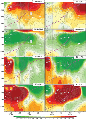
Figure 4. Budget terms of the rotational wind KE (shading; units: 10⁻³ J kg⁻¹s⁻¹) averaged within IV3 and IV4 (purple dashed boxes shown in Figure 1(a)), where the gray contours are TOT_R (units: 10⁻³ J kg⁻¹s⁻¹, with an interval of 3 × 10⁻³ J kg⁻¹s⁻¹), the solid purple line marks the top level of the cyclone, and the black-dashed lines show the maximum development stage.

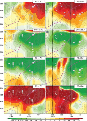
Table 1. The most favorable and detrimental factors for the enhancement of lower-tropospheric rotational wind KE within key regions IV1–IV4.

	Key region IV1	Key region IV2	Key region IV3	Key region IV4
Most favorable factors	R3	R2	R2, R3	R3
Most detrimental factors	CON	CON	CON	R1, CON