Figures & data

Figure 1. (a) The observed (black) and simulated (red/blue for control/sensitivity experiments) tracks. (b) The observed (black) and simulated (red/blue for control/sensitivity experiments) MSLPs (solid, hPa) and MSWs (dashed, m s−1), (c) surface heat fluxes (W m−2) averaged within a 100 km radius from the TC center, and (d) 850–200-hPa wind shear magnitude (solid line) and direction (dashed line) in a 600-km box centered on the TC. The SST-1 and CTL experiments are denoted by blue and red lines in each panel, respectively. The gray shading indicates the RI period.
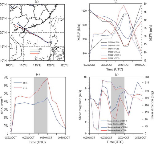
Table 1. Configuration of parameters in WRF model.
Figure 2. Observed 85-GHz microwave image of Typhoon Mujigae (a) at 0600 UTC and (b) at 1200 UTC 3 October 2015. (c–d) the simulated (CTL) maximum ice-phase mixing ratio (g kg−1) at heights of 8–10 km. The times are the same as in (a–b). (c–f) As in (c–d) but for the SST-1 experiment.
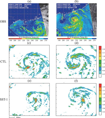
Figure 3. The averaged upper-tropospheric potential vorticity (PVU) at z = 10–15 km, horizontal wind vectors at z = 2 km and deep convection (black crosses) for the CTL simulation (left panel) at (a) 1800 UTC, (b) 2100 UTC 2 Ocotober, (c) 0000 UTC, (d) 0300 UTC, and (e) 0600 UTC 3 October. (f–j) As in (a–e) but for the SST-1 experiment (right panel).

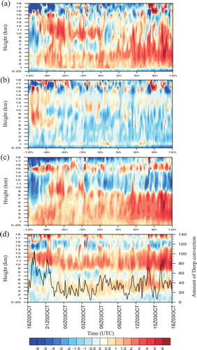
Figure 4. Time–height series of the potential vorticity budget (PVU h−1) from −12 h to 12 h relative to the RI onset for the CTL experiment. (a) PV tendency; (b) HA term; (c) DH term; (d) VA term. The black line superposed in (d) denotes the amount of deep convection.
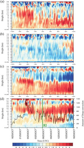
Figure 5. Time–height series of the potential vorticity budget (PVU h−1) from −12 h to 12 h relative to the RI onset for the SST-1 run. (a) PV tendency; (b) HA term; (c) DH term; (d) VA term. The black line superposed in (d) denotes the amount of deep convection.