CAS FGOALS-f3-L model dataset descriptions for CMIP6 DECK experiments

Figures & data

Table 1. Model configurations of CAS FGOALS-f3-L

Model configuration	FGOALS-f3-L
Atmosphere	FAMILv2.2 Resolution: C96 (1° × 1°) L32 (Zhou et al. 2015; Bao et al. 2019; He et al. 2019; Li et al. 2019)
Ocean	LICOM3 Resolution: Triple grid (1° × 1°) L30 (Liu et al. 2012; Li et al. 2017;)
Land	CLM4.0 Resolution: 1° × 1° (Lawrence et al. 2011)
Sea ice	CICE4.0 Resolution: 1° × 1° (Hunke et al. 2010)
Coupler	NCAR Coupler7 (Craig, Vertenstein, and Jacob 2011)

Table 2. Experiment designs

experiment_id	Variant_label	Restart time	Years of integration	Experiment design	DOI for experiment_id
piControl	r1i1p1f1	600	561	Free coupled model run with all the external forcings fixed as their values in 1850. The first 599 years of integration are taken as the spin-up time and the model outputs after 600 model years are submitted.	http://doi.10.22033/ESGF/CMIP6.3447
abrupt-4×CO2	r1i1p1f1	600	160	Restart run from 1 January in model-year 600 of piControl. CO2 prescribed as four times that in piControl. All other external forcings identical to piControl.	http://doi.10.22033/ESGF/CMIP6.3176
	r2i1p1f1	650	160	Same as r1i1p1f1 but with a restart from 1 January in model-year 650 of piControl.
	r3i1p1f1	700	160	Same as r1i1p1f1 but with a restart from 1 January in model-year 700 of piControl.
1pctCO2	r1i1p1f1	600	160	Restart run from 1 January in model-year 600 of piControl. CO2 prescribed to increase 1% yr^−1. All other external forcings identical to piControl.	http://doi.10.22033/ESGF/CMIP6.3054
	r2i1p1f1	650	160	As in r1i1p1f1 but with a restart from 1 January in model-year 650 of piControl.
	r3i1p1f1	700	160	As in r1i1p1f1 but with a restart from 1 January in model-year 700 of piControl.

Table 3. External forcing settings in piControl, abrupt-4×CO2, and 1pctCO2

External forcing	Description
GHGs	Fixed as their global mean values in 1850: CO2: 284.3 ppm in piControl 1137.2 ppm in abrupt-4×CO2 1% yr^−1 increase from 284.3 ppm in 1pctCO2 CH4: 808.2 ppb N2O: 273.0 ppb CFC-11 equivalent: 0.032 ppb CFC-12 equivalent: 0.016 ppb
Solar irradiance	1360.8 W m^−2
Aerosols	Three-dimensional distributions prescribed as their values in 1850, including sulfates, sea salt, black carbon, organic carbon, and dust (Lamarque et al. 2012)
Ozone	Three-dimensional distributions prescribed as their values in 1850 (http://blogs.reading.ac.uk/ccmi/forcing-databases-in-support-of-cmip6/)

Figure 1. (a) Time series of global mean TOA net radiation (units: W m⁻²) for piControl from model-year 600 to 1160 with a global mean value of 0.31 W m⁻², standard deviation of 0.37 W m⁻² and climate trend of −0.03 W m⁻²/100 yr. (b) Time series of global mean SST for piControl from model-year 600 to 1160 with a global mean value of 16.45°C, standard deviation of 0.11°C and climate trend of 0.03°C/100 yr

Figure 2. Climate mean distribution of SST (units: °C): (a) observation (1871–1900 mean); (b) FGOALS-f3-L (600–1160 mean)

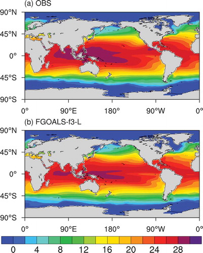
Figure 3. Climate mean distribution of precipitation (units: mm d⁻¹): (a) observation (1979–2014); (b) FGOALS-f3-L (600–1160 mean)

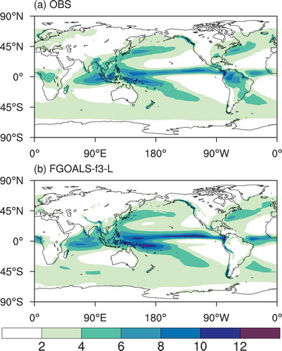
Table 4. Surface air temperature responses to abrupt quadrupling of CO₂ and 1% yr⁻¹ CO₂ increase at 150 model years

SAT responses (°C) at 150 model years	abrupt-4×CO2	1pctCO2
Ensemble mean	5.07	5.09
r1i1p1f1	5.20	5.16
r2i1p1f1	4.98	5.18
r3i1p1f1	5.04	4.95

Figure 4. Time series of global mean surface air temperature anomalies (units: °C; relative to piControl) for ensemble means of abrupt-4×CO2 and 1pctCO2, respectively. The dashed lines are the three ensemble members, respectively

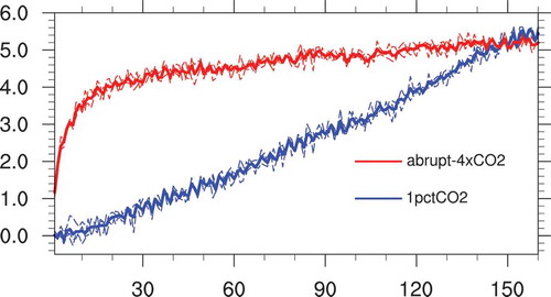
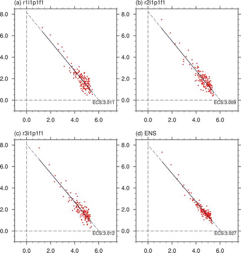
Figure 5. Climate sensitivity of CAS FGOALS-f3-L estimated from the 160-year integrations from abrupt-4×CO2 and associated piControl simulations. The abscissa is the surface air temperature anomaly (units: °C) and the vertical axis is the TOA net radiation anomaly (units: W m⁻²). The blue dashed lines are the extension lines of the regression lines. (a) r1i1p1f1; (b) r2i1p1f1; (c) r3i1p1f1; (d) ensemble mean

Zhou, L., Q. Bao, Y. M. Liu, G. X. Wu, W. C. Wang, X. C. Wang, B. He, H. Y. Yu, and J. D. Li. 2015. “Global Energy and Water Balance: Characteristics from Finite‐volume Atmospheric Model of the IAP/LASG (FAMIL1).” Journal of Advances in Modeling Earth Systems 7 (1): 1–20. doi:10.1002/2014ms000349.

 Web of Science ®Google Scholar

Bao, Q., X. F. Wu, J. X. Li, L. Wang, B. He, X. C. Wang, Y. M. Liu, and G. X. Wu. 2019. “Outlook for ElNino and the Indian Ocean Dipole in Autumn-winter 2018–2019.” (In Chinese). Chinese Science Bulletin 64 (1): 73–78. doi:10.1360/N972018-00913.

 Google Scholar

He, B., Q. Bao, X. C. Wang, L. J. Zhou, X. F. Wu, Y. M. Liu, G. X. Wu, et al. 2019. “CAS FGOALS-f3-L Model Datasets for CMIP6 Historical Atmospheric Model Intercomparison Project Simulation.” Advances in Atmospheric Sciences 36 (8): 771–778. doi:10.1007/s00376-019-9027-8.

 Web of Science ®Google Scholar

Li, J. X., Q. Bao, Y. M. Liu, G. X. Wu, L. Wang, B. He, X. C. Wang, and J. D. Li. 2019. “Evaluation of FAMIL2 in Simulating the Climatology and Seasonal-to-interannual Variability of Tropical Cyclone Characteristics.” Journal of Advances in Modeling Earth Systems. doi:10.1029/2018MS001506.

 Web of Science ®Google Scholar

Liu, H., P. Lin, Y. Yu, and X. Zhang. 2012. “The Baseline Evaluation of LASG/IAP Climate System Ocean Model (LICOM) Version 2.” Acta Meteorologica Sinica 26: 318–329. doi:10.1007/s13351-012-0305-y.

 Web of Science ®Google Scholar

Li, X., Y. Yu, H. Liu, and P. Lin. 2017. “Sensitivity of Atlantic Meridional Overturning Circulation to the Dynamical Framework in an Ocean General Circulation Model.” Journal of Meteorological Research 31: 490–501. doi:10.1007/s13351-017-6109-3.

 Web of Science ®Google Scholar

Lawrence, D. M., K. W. Oleson, M. G. Flanner, P. E. Thornton, S. C. Swenson, P. J. Lawrence, X. B. Zeng, et al. 2011. “Parameterization Improvements and Functional and Structural Advances in Version 4 of the Community Land Model.” Journal of Advances in Modeling Earth Systems. 3: M03001. doi:10.1029/2011MS00045.

 Web of Science ®Google Scholar

Hunke, E. C., W. H. Lipscomb, A. K. Turner, N. Jeffery, and S. Elliott. 2010. “CICE: The Los Alamos Sea Ice Model Documentation and Software User’s Manual Version 4.1 LA-CC-06-012.” T-3 Fluid Dynamics Group, Los Alamos National Laboratory, 675.

 Google Scholar

Craig, A., M. Vertenstein, and R. Jacob. 2011. “A New Flexible Coupler for Earth System Modeling Developed for CCSM4 and CESM1.” International Journal of High Performance Computing Applications 26: 31–42. doi:10.1177/1094342011428141.

 Web of Science ®Google Scholar

Lamarque, J.-F., L. K. Emmons, P. G. Hess, D. E. Kinnison, S. Tilmes, F. Vitt, C. L. Heald, et al. 2012. “CAM-chem: Description and Evaluation of Interactive Atmospheric Chemistry in the Community Earth System Model.” Geoscientific Model Development 5 (2): 369–411. doi:10.5194/gmd-5-369-2012.

 Web of Science ®Google Scholar

Data availability statement

The data that support the findings of this study are available from https://esgf-node.llnl.gov/projects/cmip6/