Properties of summer radiation and aerosols at Xinzhou, a suburban site on the North China Plain

Figures & data

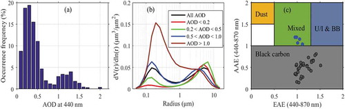
Figure 1. Location of Xinzhou (red dot), ~450 km southwest of Beijing (BJ; red rectangle). The color bar represents the altitude, which is 700 m at Xinzhou

Table 1. Main specifications of the six radiometers deployed at Xinzhou

	SW	LW	Direct	Diffuse	PAR	UVA/UVB
Spectral range (µm)	0.2–3.6	4.5–42	0.2–4	0.2–3.6	0.4–0.7	0.315–0.4/0.28–0.315
Response time	< 5 s	< 18 s	< 5 s	< 5 s	< 1 µs	< 1.5 s
Nonlinearity	< 0.2%	< 1%	<0.2%	< 0.2%	< 1%	< 1%

Table 2. Summary of the daily maximum and the daily average over four months for the seven radiation parameters

	SW	LW	Direct	Diffuse	PAR	UVA	UVB
Daily maximum (W m^−2)	689.9	392.6	352.0	339.8	293.6	11.5	1.4
Daily averages (W m^−2)	353.5	375.2	216.9	186.8	150.1	5.8	0.6

Figure 2. Diurnal evolutions and their standard deviations for different radiation types: (a) SW; (b) LW; (c) direct; (d) diffuse; (e) PAR; and (f) UVA and UVB

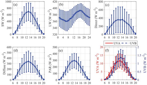
Figure 3. Monthly variations and their standard deviations for different radiation types: (a) SW; (b) LW; (c) direct; (d) diffuse; (e) PAR; and (f) UVA and UVB. The average of each parameter during all months is also shown. The color bar in each panel represents the number of observation days

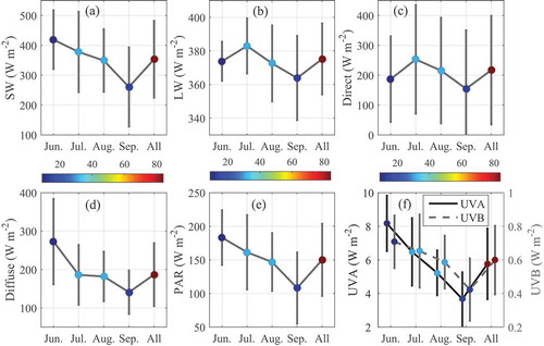
Figure 4. (a) Occurrence frequency of AOD at 440 nm derived from the direct sun algorithm. (b) Aerosol volume size distributions for all AOD (black line) and sorted by different AOD bins, i.e., < 0.2 (red line), 0.2–0.5 (green line), 0.5–1.0 (blue line), and >1.0 (brown line). (c) Distributions of AAE as a function of EAE for the aerosol cases with AOD > 0.4 at 440 nm; the areas with different colors mark the extent of different aerosol types

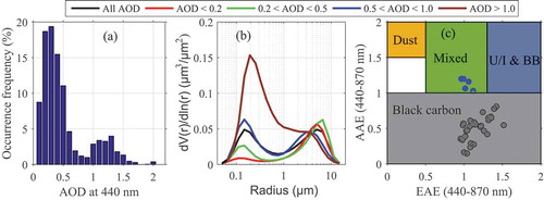
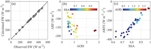
Figure 5. (a) The inversion algorithm–calculated SW as a function of the observed SW. The black line denotes the 1:1 line. (b) Scatterplot of instantaneous ARF at the BOA as a function of AOD and (c) ARFE as a function of SSA derived from the aerosol inversion algorithm. The color bar in panels (b, c) presents the values of SSA and AOD for the data points, respectively