Figures & data
Figure 1. RBFN with a single output unit.
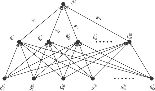
Figure 2. Univariate function interpolation using conventional and new RBFNs. Ten (for the conventional RBFN, left) and five (for the new RBFN, with known gradient too, right) training points (b,τ ), where τ (b)= b2 + 10(1- cos ( 2 π b)), have been used. After training the two RBFNs, the interpolated function is plotted along with the target–function curve.
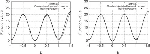
Figure 3. Two parameter (M = 2) Ackley function: distribution of the N = 50 (new RBFN, left) and N = 100 (conventional RBFN, right) randomly chosen training patterns and the point-free circle around the optimal solution.
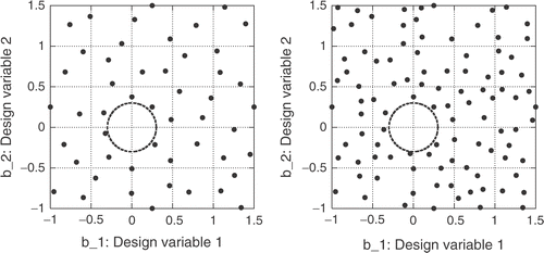
Figure 4. Two parameter (M = 2) Ackley function: Iso-area contours: (a) predicted by the new RBFN (top-left), (b) predicted by the conventional RBFN, i.e. without taking into account gradient information (top-right), and (c) analytically computed (bottom).
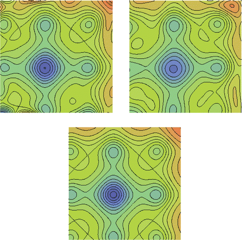
Figure 5. Ten parameter (M = 10) Ackley function: convergence history.
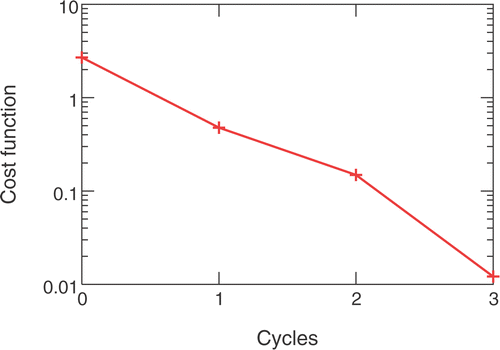
Figure 6. Two-objective function minimization: The exact Pareto front (dashed line) and that computed using the RBFN (marks).
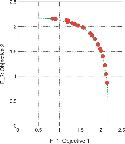
Figure 7. Two-objective function minimization: Response surfaces for the first (left column) and second (right column) objective functions. The exact shapes (top), the ones computed using the new RBFN (mid) and those produced using a conventional RBFN (bottom) are shown.
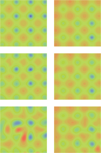
Figure 8. Inverse design of a 3D peripheral compressor cascade: Mach number distribution over the reference cascade which corresponds to the pressure distribution imposed as target.
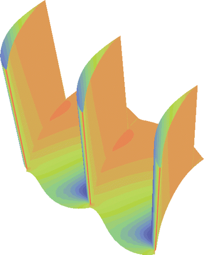
Figure 9. Inverse design of a 3D peripheral compressor cascade: Objective function value for the initial training patterns, sorted in descending order.
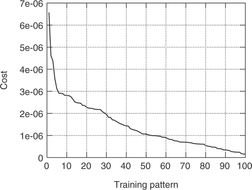
Figure 10. Inverse design of a 3D peripheral compressor cascade: Convergence history. The CPU cost associated with each cycle is that of a single evaluation (numerical solution of the flow and adjoint equations, i.e. two equivalent flow solutions) since the cost of retraining the RBFN and searching through EAs is almost negligible. The major burden is that of evaluating the starting training database (100 points in the search space, i.e. 200 equivalent flow solutions), not included in this figure.
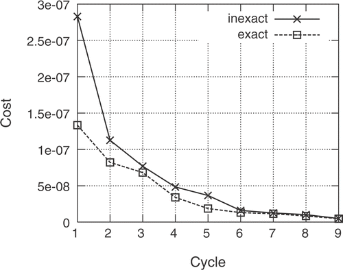
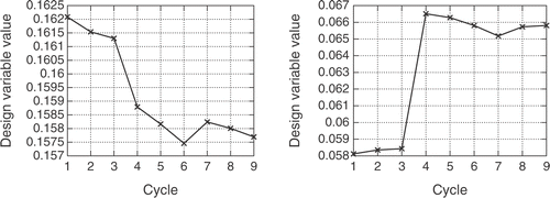
Figure 11. Inverse design of a 3D peripheral compressor cascade: Monitoring of the second and sixth design variable values during the nine optimization cycles.