Estimation of thermal resistance distributions for die-attach testing in microelectronics

Figures & data

Figure 1. Semiconductor chip attached to a heat spreader.

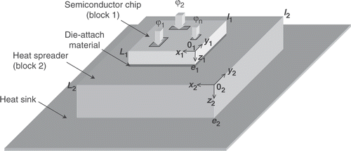
Figure 2. Thermal boundary conditions considered for the block 1 in multiblock decomposition (cross-sectional view).

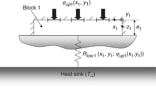
Figure 3. Thermal boundary conditions considered for the block 2 in multi-block decomposition (cross-sectional view).

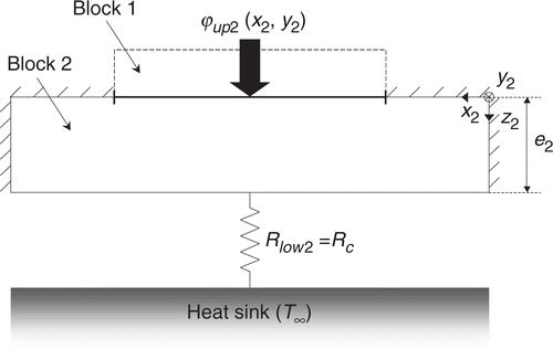
Figure 4. Principle of the iterative process for solving the 3D steady-state heat conduction direct problem.

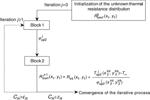
Figure 5. Heat source configuration on the upper face of the block 1 for the validation of the direct problem.

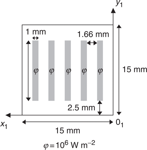
Figure 6. Interface thermal resistance distribution (K m² W⁻¹): R_int(x₁,y₁) = 0.5 × sin(x₁.y₁) − validation of the direct problem.

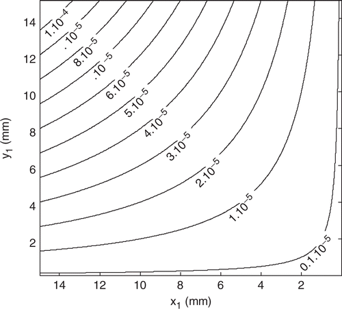
Table 1. Thermal properties and dimensions of the microelectronic device for the validation of the direct problem

Material	λ (W m^−1 K^−1)	L (mm)	l (mm)	e (mm)
GaAs (block 1)	44	15	15	0.5
CuW (block 2)	150	30	30	5

Figure 7. Validation of the direct problem–temperature profiles on the upper face of the block 1: (a) for y₁ = 7.5 mm, (b) for x₁ = 7.5 mm.

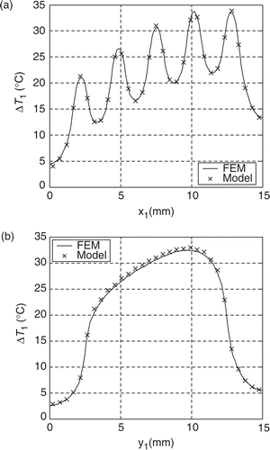
Figure 8. Examples of parametrization of the interface thermal resistance distribution: (a) 4-zone partition, (b) 25-zone partition, (c) 64-zone partition.

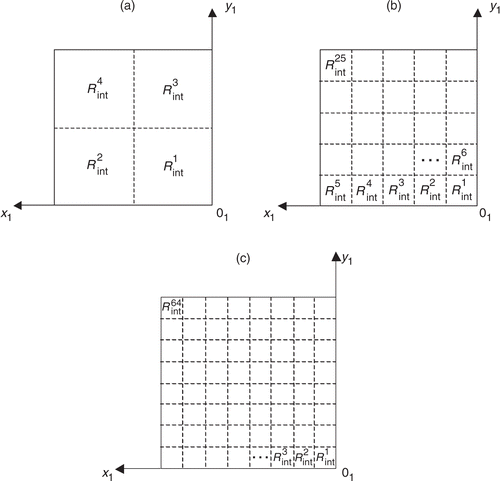
Figure 9. Exact interface thermal resistance distributions (Km² W⁻¹) investigated in the numerical experiments.

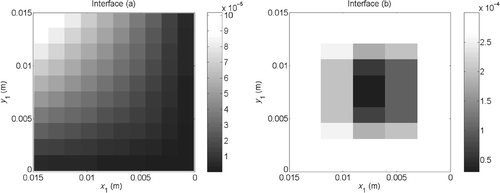
Table 2. Spatial characteristics of the exact interface thermal resistance distributions

Interface type	Interface thermal resistance distribution (K m^2 W^−1)
(a)	Rint = 0.5 × sin(x1, y1)
(b)	Rint = 3 × 10^−5 if 0.4L1 < x1 < 0.6L1 and 0.4l1 < y1 < 0.6l1
	Rint = 6 × 10^−5 if 0.4L1 < x1 < 0.6L1 and 0.6l1 ≤ y1 < 0.7l1
	Rint = 7 × 10^−5 if 0.4L1 < x1 < 0.6L1 and 0.3l1 < y1 ≤ 0.4l1
	Rint = 1 × 10^−4 if 0.2L1 < x1 ≤ 0.4L1 and 0.3l1 < y1 < 0.7l1
	Rint = 1.85 × 10^−4 if 0.4L1 < x1 < 0.6L1 and 0.2l1 < y1 ≤ 0.3l1 or 0.7l1 ≤ y1 < 0.8l1
	Rint = 2 × 10^−4 if 0.2L1 < x1 ≤ 0.4L1 and 0.2l1 < y1 ≤ 0.3l1 or 0.7l1 ≤ y1 < 0.8l1
	Rint = 2 × 10^−4 if 0.6L1 ≤ x1 < 0.8L1 and 0.3l1 < y1 < 0.7l1
	Rint = 2.5 × 10^−4 if 0.6L1 ≤ x1 < 0.8L1 and 0.2l1 < y1 ≤ 0.3l1 or 0.7l1 ≤ y1 < 0.8l1
	Rint = 3 × 10^−4 elsewhere

Figure 10. Heat source configurations on the upper face of the block 1 investigated in the numerical experiments.

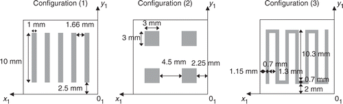
Figure 11. Sensitivity coefficients distribution (Wm⁻²) of η(β) to the component n°33 of β computed for the HSC (1) and .

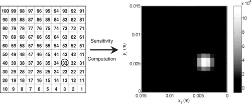
Figure 12. Average sensitivity coefficients profiles computed for the three HSC and .

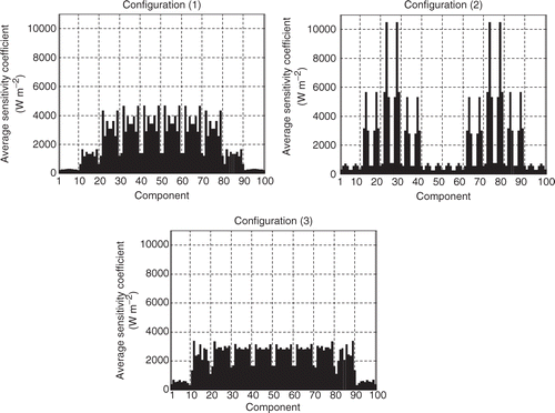
Figure 13. Evolution of the estimated distributions (Km² W⁻¹) (interface (a), HSC (1), and σ = 0): (a) 5 iterations, (b) 20 iterations, (c) 50 iterations, (d) 100 iterations.

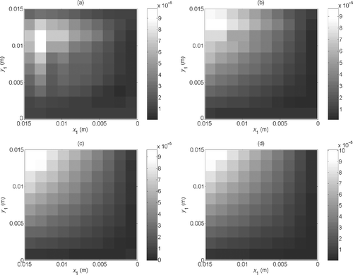
Figure 14. Evolution of the functional J for the estimation of the interface (a) with the three HSC, and σ = 0.1 K.

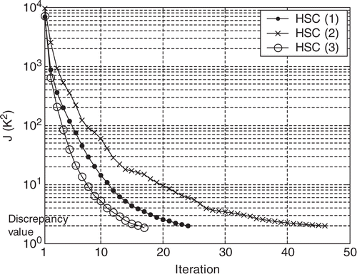
Figure 15. Evolution of the functional J for the estimation of the interface (b) with the three HSC, and σ = 0.1 K.

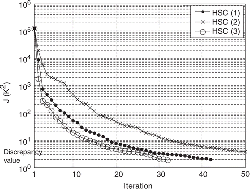
Figure 16. Components of β for the estimation of the interface (a) with the HSC (3) and σ = 0.1 K.

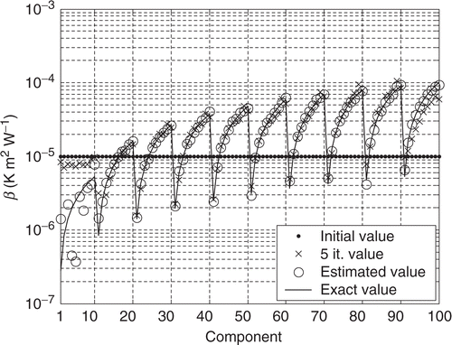
Figure 17. Components of β for the estimation of the interface (b) with the HSC (3) and σ = 0.1 K.

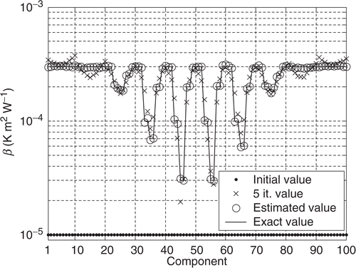
Figure 18. Relative error due to measurement errors for the estimation of the interface (a) with the HSC (3) and σ = 0.1 K.

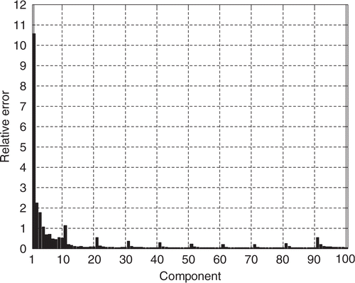
Figure 19. Relative error due to measurement errors for the estimation of the interface (b) with the HSC (3) and σ = 0.1 K.

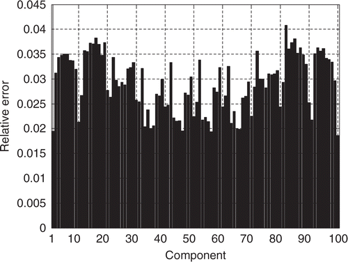
Figure 20. Evolution of the functional J for the estimation of the interface (a) with the HSC (1), σ = 0.1 K, and different update parameters K.

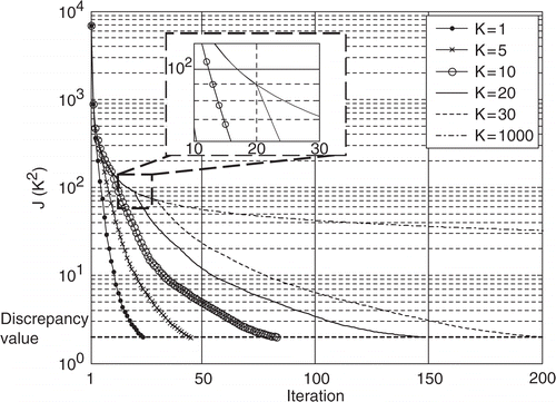
Figure 21. Computation time of the estimation of the interface (a) with the HSC (1), σ = 0.1 K, as a function of the update parameter K.

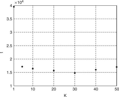
Figure 22. Refinement levels of the interface grid.

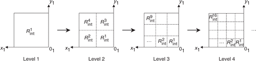
Figure 23. Interface thermal resistance distribution (K m² W⁻¹) searched to illustrate the refinement method.

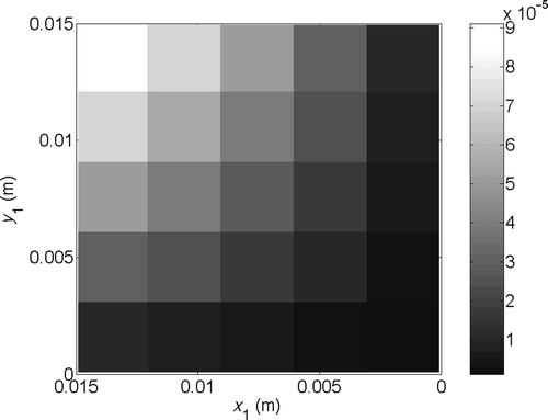
Figure 24. Estimated distributions (K m² W⁻¹) for the first six refinement levels with the HSC (1), σ = 0.1 K and .

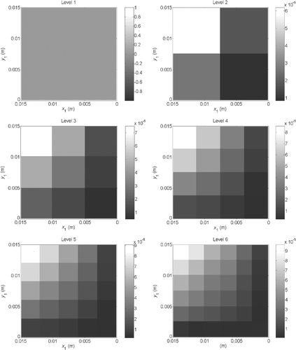
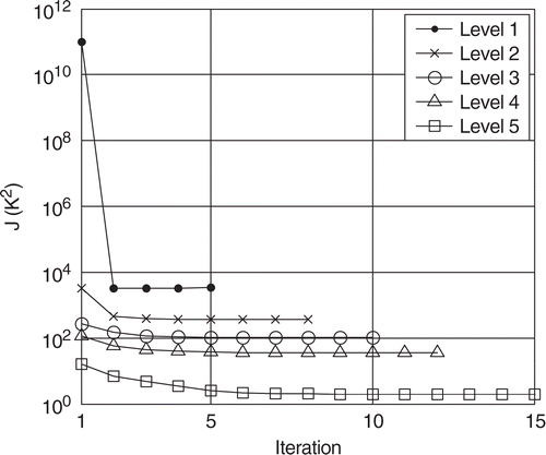
Figure 25. Evolution of the functional J for the first six refinement levels with the HSC (1), σ = 0.1 K and .

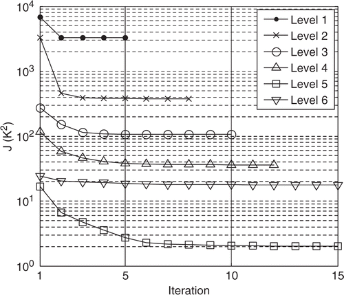
Figure 26. Evolution of the functional J without refinement of the interface grid with the HSC (1), σ = 0.1 K and .

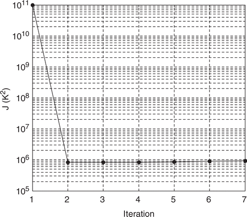
Figure 27. Evolution of the functional J for the first five refinement levels with the HSC (1), σ = 0.1 K and .