193
Views
7
CrossRef citations to date
0
Altmetric
Original Articles

Application of a GEO + SA hybrid optimization algorithm to the solution of an inverse radiative transfer problem

, , &
Pages 321-334 | Received 16 Apr 2007, Accepted 30 Nov 2007, Published online: 24 Mar 2009

Figures & data

Figure 1. The canonical variant of GEO.

Figure 1. The canonical variant of GEO.

Figure 2. Scheduling examples for γ.

Figure 2. Scheduling examples for γ.

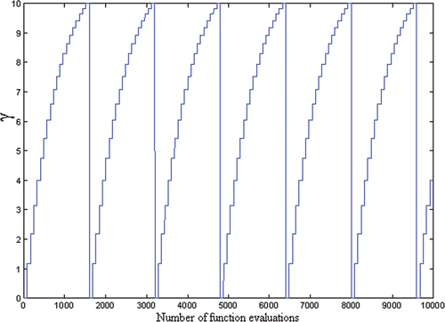
Figure 3. Cyclic scheduling example.

Figure 3. Cyclic scheduling example.

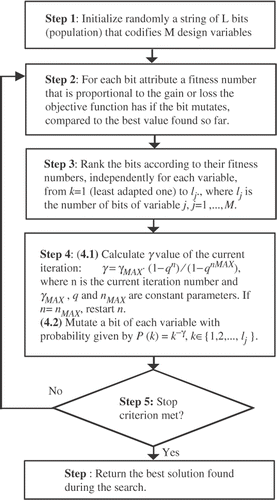
Figure 4. GEO + SA algorithm.

Figure 4. GEO + SA algorithm.

Table 1. Exact values of the radiative properties.

Figure 5. Average of the best values of the objective function, as a function of the number of function evaluations for Case 1, without noise.
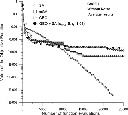
Figure 5. Average of the best values of the objective function, as a function of the number of function evaluations for Case 1, without noise.

Figure 6. Average of the best values of the objective function, as a function of the number of function evaluations for Case 1, with noise.
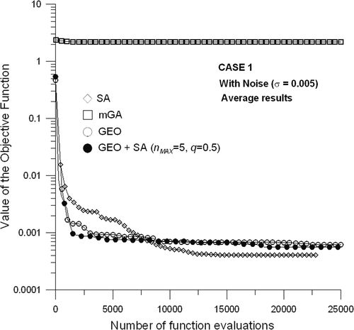
Figure 6. Average of the best values of the objective function, as a function of the number of function evaluations for Case 1, with noise.

Table 2. Worst, average and best estimates for Case 1.

Figure 7. Average of the best values of the objective function, as a function of the number of function evaluations for Case 2, without noise.
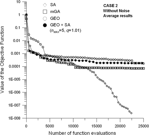
Figure 7. Average of the best values of the objective function, as a function of the number of function evaluations for Case 2, without noise.

Table 3. Worst, average and best estimates for Case 2.

Figure 8. Average of the best values of the objective function, as a function of the number of function evaluations for Case 2, with noise.
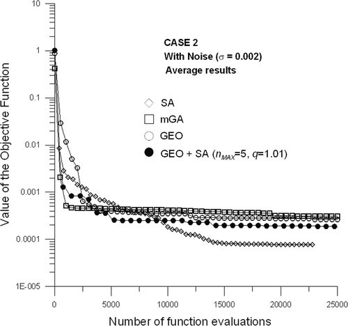
Figure 8. Average of the best values of the objective function, as a function of the number of function evaluations for Case 2, with noise.

Figure 9. Average of the best values of the objective function, as a function of the number of function evaluations for Case 3, without noise.
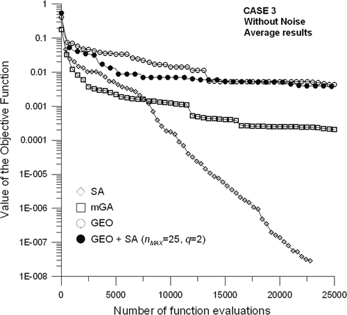
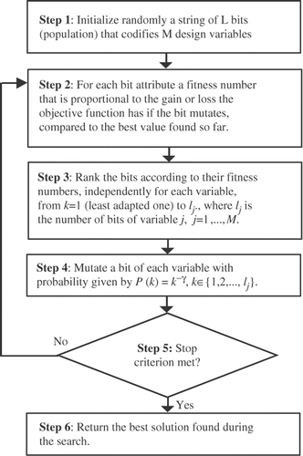
Figure 9. Average of the best values of the objective function, as a function of the number of function evaluations for Case 3, without noise.
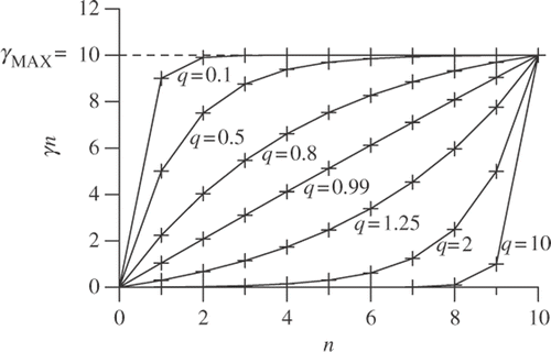
Table 4. Worst, average and best estimates for Case 3.

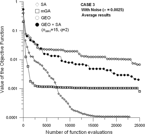
Figure 10. Average of the best values of the objective function, as a function of the number of function evaluations for Case 3, with noise.

Figure 10. Average of the best values of the objective function, as a function of the number of function evaluations for Case 3, with noise.

Reprints and Corporate Permissions

Please note: Selecting permissions does not provide access to the full text of the article, please see our help page How do I view content?

To request a reprint or corporate permissions for this article, please click on the relevant link below:

Academic Permissions

Please note: Selecting permissions does not provide access to the full text of the article, please see our help page How do I view content?

Obtain permissions instantly via Rightslink by clicking on the button below:

If you are unable to obtain permissions via Rightslink, please complete and submit this Permissions form. For more information, please visit our Permissions help page.