248
Views
9
CrossRef citations to date
0
Altmetric
Original Articles

Dynamic observers based on Green's functions applied to 3D inverse thermal models

, &
Pages 743-761 | Received 16 Apr 2007, Accepted 30 Nov 2007, Published online: 18 Sep 2008

Figures & data

Figure 1. One-dimensional thermal model.

Figure 1. One-dimensional thermal model.

Figure 2. Spatially discretized system using finite volume method Citation10.
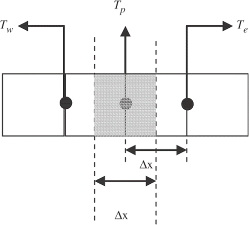
Figure 2. Spatially discretized system using finite volume method Citation10.

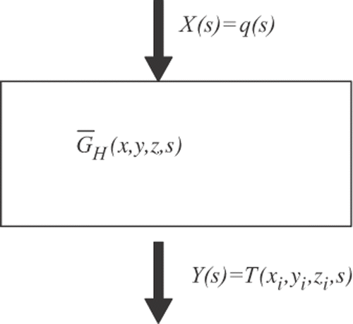
Figure 3. Frequency-domain block diagram Citation8.
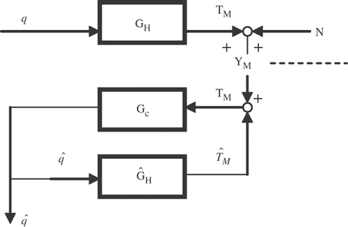
Figure 3. Frequency-domain block diagram Citation8.

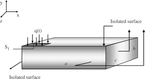
Figure 4. 3D-transient thermal model.

Figure 4. 3D-transient thermal model.

Figure 5. Dynamic thermal model system.

Figure 5. Dynamic thermal model system.

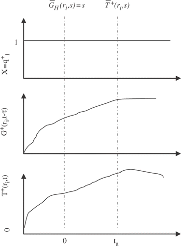
Figure 6. Calculation of cross correlation of GH.

Figure 6. Calculation of cross correlation of GH.

Figure 7. Experimental temperatures simulated numerically at x = L, with εi = 0.0, within ±0.5°C, within ±1.0°C.: sinusoidal heat flux.
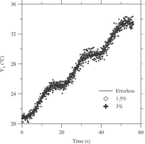
Figure 7. Experimental temperatures simulated numerically at x = L, with εi = 0.0, within ±0.5°C, within ±1.0°C.: sinusoidal heat flux.

Figure 8. Experimental temperatures simulated numerically at x = L, with εi = 0.0, within ±0.5°C, within ±1.0°C.: triangular heat flux.
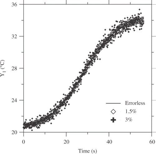
Figure 8. Experimental temperatures simulated numerically at x = L, with εi = 0.0, within ±0.5°C, within ±1.0°C.: triangular heat flux.

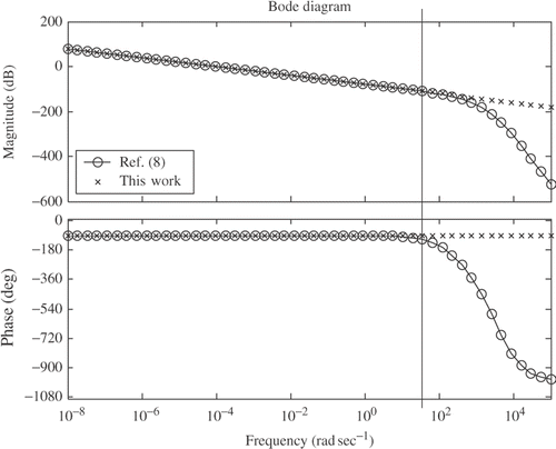
Figure 9. Modulus and phase of heat transfer function, GH.

Figure 9. Modulus and phase of heat transfer function, GH.

Figure 10. Heat flux estimation using temperature data without noise error. (a) sinusoidal; (b) triangular.
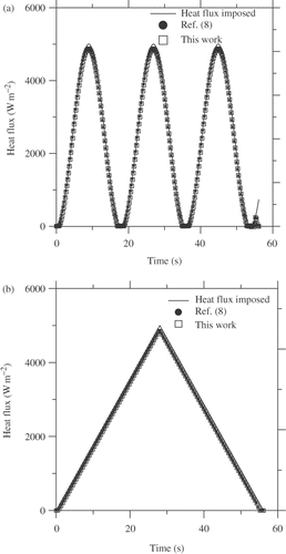
Figure 10. Heat flux estimation using temperature data without noise error. (a) sinusoidal; (b) triangular.

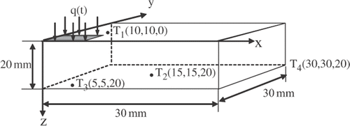
Figure 11. 3D thermal model test with simulated temperature sensor locations.

Figure 11. 3D thermal model test with simulated temperature sensor locations.

Figure 12. Heat flux estimation using simulated temperatures, εi within ±1.5°C: (a) flux sinusoidal; (b) flux triangular (test 3D).
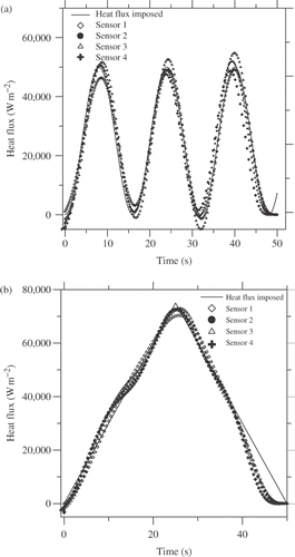
Figure 12. Heat flux estimation using simulated temperatures, εi within ±1.5°C: (a) flux sinusoidal; (b) flux triangular (test 3D).

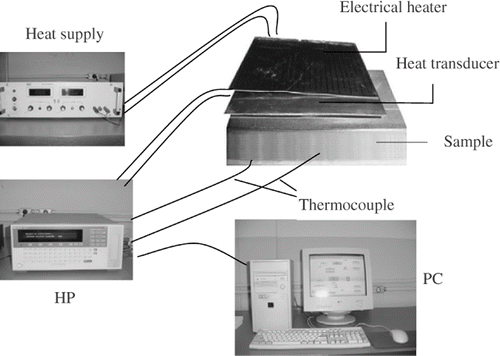
Figure 13. Apparatus experimental scheme.

Figure 13. Apparatus experimental scheme.

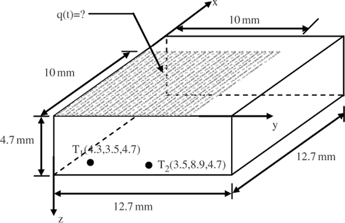
Figure 14. Thermocouple sensor location and geometric sample description.

Figure 14. Thermocouple sensor location and geometric sample description.

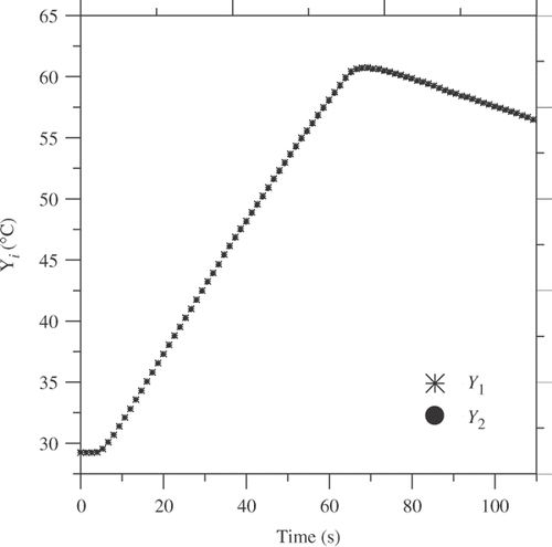
Figure 15. Experimental temperature evolution of Y1(t) and Y2(t).

Figure 15. Experimental temperature evolution of Y1(t) and Y2(t).

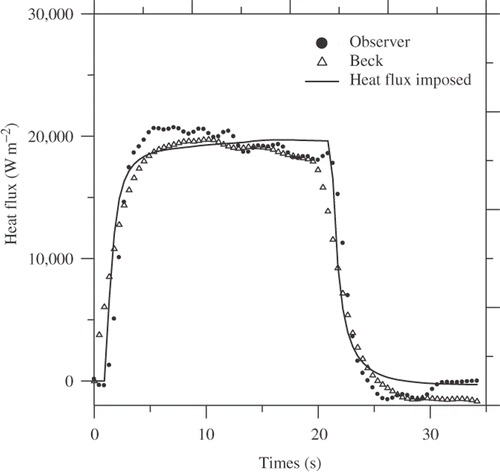
Figure 16. Comparison between the measured and estimated heat flux using Y1(t).

Figure 16. Comparison between the measured and estimated heat flux using Y1(t).

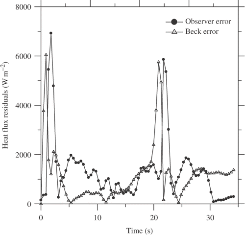
Figure 17. Residuals of heat flux estimated and measured.

Figure 17. Residuals of heat flux estimated and measured.

Figure 18. Zero-memory non-linear system Citation16.

Figure 18. Zero-memory non-linear system Citation16.

Figure 19. Finite-memory non-linear system with linear systems before and after the zero-memory non-linear system Citation16.

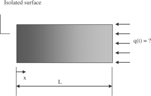
Figure 19. Finite-memory non-linear system with linear systems before and after the zero-memory non-linear system Citation16.
Reprints and Corporate Permissions

Please note: Selecting permissions does not provide access to the full text of the article, please see our help page How do I view content?

To request a reprint or corporate permissions for this article, please click on the relevant link below:

Academic Permissions

Please note: Selecting permissions does not provide access to the full text of the article, please see our help page How do I view content?

Obtain permissions instantly via Rightslink by clicking on the button below:

If you are unable to obtain permissions via Rightslink, please complete and submit this Permissions form. For more information, please visit our Permissions help page.