331
Views
31
CrossRef citations to date
0
Altmetric
Original Articles

Recovering the source term in a linear diffusion problem by the method of fundamental solutions

, , , , &
Pages 1005-1021 | Received 16 Apr 2007, Accepted 30 Nov 2007, Published online: 08 Nov 2008

Figures & data

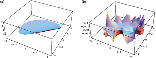
Figure 1. Counter-example on uniqueness: the solution τ (a) which verifies null Cauchy data and the source gτ (b).
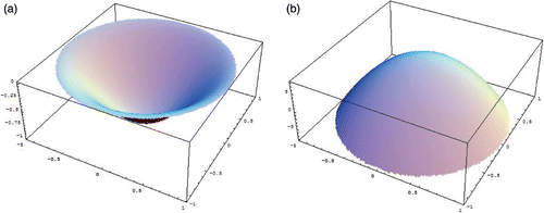
Figure 1. Counter-example on uniqueness: the solution τ (a) which verifies null Cauchy data and the source gτ (b).

Figure 2. Counter-example: solution on the annulus (a) (a, b) = (1, 2), (b) .

Figure 2. Counter-example: solution on the annulus (a) (a, b) = (1, 2), (b) .

Figure 3. Counter-example: radial profile of the solution TA and the characteristic source.

Figure 3. Counter-example: radial profile of the solution TA and the characteristic source.

Figure 4. Distribution of points in two geometries: (a) circle with radius 1, (b) a peanut shape. Note: Domain collocation points zi (black dots), boundary collocation points xi (grey dots) and external point sources yj (bold black dots).
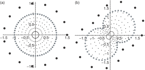
Figure 4. Distribution of points in two geometries: (a) circle with radius 1, (b) a peanut shape. Note: Domain collocation points zi (black dots), boundary collocation points xi (grey dots) and external point sources yj (bold black dots).

Figure 5. (a) The computed g and (b) The absolute error of the source, in Simulation 1.

Figure 5. (a) The computed g and (b) The absolute error of the source, in Simulation 1.

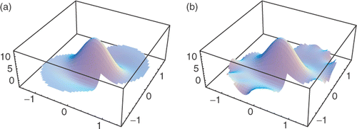
Figure 6. Simulation 2: (a) The exact g, and (b) The computed g with noisy data.

Figure 6. Simulation 2: (a) The exact g, and (b) The computed g with noisy data.

Figure 7. Simulation 3: Reconstruction of χω1. (a) The choice of collocation points; (b) the approximation of T.
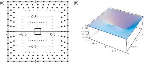
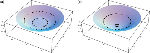
Figure 7. Simulation 3: Reconstruction of χω1. (a) The choice of collocation points; (b) the approximation of T.
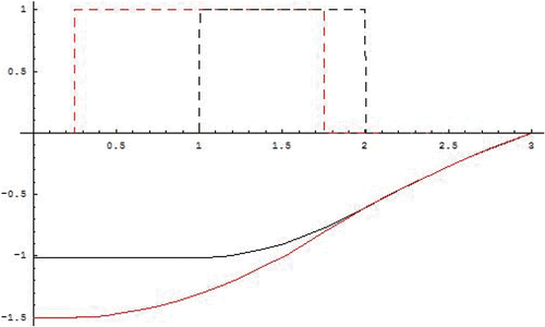
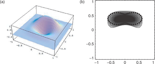
Figure 8. Simulation 3: Reconstruction of χω1. (a) the approximation of g = χω1; (b) A density plot cutted at half amplitude of and the comparison with ω1 (dotted boundary).

Figure 8. Simulation 3: Reconstruction of χω1. (a) the approximation of g = χω1; (b) A density plot cutted at half amplitude of and the comparison with ω1 (dotted boundary).

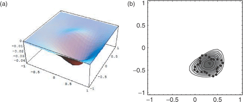
Figure 9. Simulation 4: Reconstruction of χω2. (a) The approximation ; (b) A density plot cutted at half amplitude of and the comparison with ω2 (dotted boundary).

Figure 9. Simulation 4: Reconstruction of χω2. (a) The approximation ; (b) A density plot cutted at half amplitude of and the comparison with ω2 (dotted boundary).

Reprints and Corporate Permissions

Please note: Selecting permissions does not provide access to the full text of the article, please see our help page How do I view content?

To request a reprint or corporate permissions for this article, please click on the relevant link below:

Academic Permissions

Please note: Selecting permissions does not provide access to the full text of the article, please see our help page How do I view content?

Obtain permissions instantly via Rightslink by clicking on the button below:

If you are unable to obtain permissions via Rightslink, please complete and submit this Permissions form. For more information, please visit our Permissions help page.