230
Views
6
CrossRef citations to date
0
Altmetric
Original Articles

Reduced modelling through identification on 2D incompressible laminar flows

, , , &
Pages 303-319 | Received 16 Apr 2007, Accepted 20 Jan 2008, Published online: 24 Mar 2009

Figures & data

Figure 1. The identification principle.

Figure 1. The identification principle.

Figure 2. The computation grid with N = 15876 nodes and the boundary conditions.

Figure 2. The computation grid with N = 15876 nodes and the boundary conditions.

Table 1. Maximal and mean velocity value of the identification data in the test case 1.

Table 2. Influence of RM order.

Figure 3. u velocity field of the DM (left) and the RM n = 8 (right) for Re = 1000. Available in colour online.
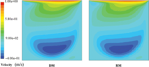
Figure 3. u velocity field of the DM (left) and the RM n = 8 (right) for Re = 1000. Available in colour online.
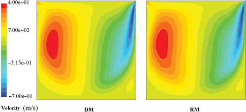
Figure 4. v velocity field of the DM (left) and the RM n = 8 (right) for Re = 1000. Available in colour online.

Figure 4. v velocity field of the DM (left) and the RM n = 8 (right) for Re = 1000. Available in colour online.

Figure 5. Stream function ψ fields of the DM (left) and the RM n = 8 (right) for Re = 1000. Available in colour online.
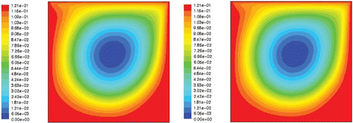
Figure 5. Stream function ψ fields of the DM (left) and the RM n = 8 (right) for Re = 1000. Available in colour online.

Figure 6. Vorticity ω fields of the DM (left) and the RM n = 8 (right) for Re = 1000. Available in colour online.
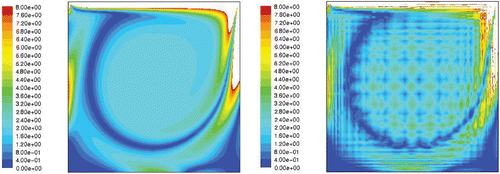
Figure 6. Vorticity ω fields of the DM (left) and the RM n = 8 (right) for Re = 1000. Available in colour online.

Table 3. Maximal and mean value of the DM velocity field at Re = 1000 and the corresponding errors of the RM n = 8.

Figure 7. Comparison of DM and RM: velocity profiles of u component at x = 0.5d. Available in colour online.
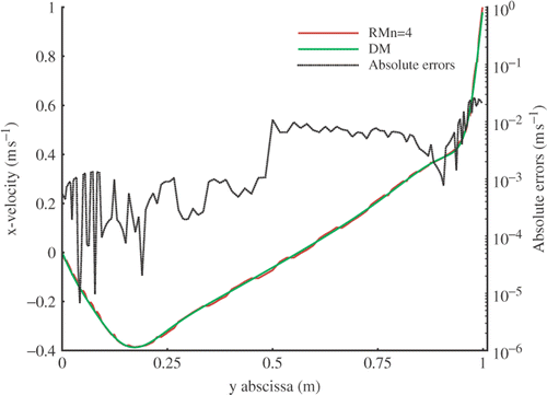
Figure 7. Comparison of DM and RM: velocity profiles of u component at x = 0.5d. Available in colour online.

Figure 8. Comparison of DM and RM velocity profiles of v component at y = 0.5d. Available in colour online.
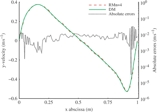
Figure 8. Comparison of DM and RM velocity profiles of v component at y = 0.5d. Available in colour online.

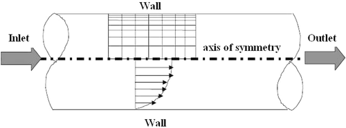
Figure 9. Geometry and mesh of the pipe.

Figure 9. Geometry and mesh of the pipe.

Figure 10. Centerline axial velocity (left) and axial outlet velocity profile (right) of the DM for Re = 100.
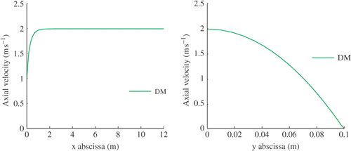
Figure 10. Centerline axial velocity (left) and axial outlet velocity profile (right) of the DM for Re = 100.
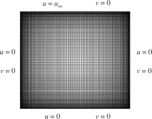
Table 4. Maximal and mean velocity value of the identification data in test case 2.

Table 5. Influence of RM order.

Table 6. Maximal and mean value of the DM velocity field at Re = 400 and the corresponding errors of the RM n = 6.

Table 7. Maximal and mean value of the DM velocity field at Re = 800 and the corresponding errors of the RM n = 6.

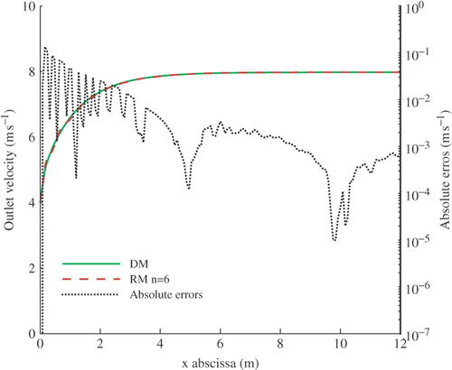
Figure 11. Centerline axial velocity profiles of the DM and the RM of order n = 6 for Re = 400.

Figure 11. Centerline axial velocity profiles of the DM and the RM of order n = 6 for Re = 400.

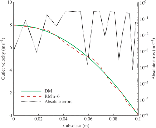
Figure 12. Outlet axial velocity profiles of the DM and the RM of order n = 6 for Re = 400.

Figure 12. Outlet axial velocity profiles of the DM and the RM of order n = 6 for Re = 400.

Reprints and Corporate Permissions

Please note: Selecting permissions does not provide access to the full text of the article, please see our help page How do I view content?

To request a reprint or corporate permissions for this article, please click on the relevant link below:

Academic Permissions

Please note: Selecting permissions does not provide access to the full text of the article, please see our help page How do I view content?

Obtain permissions instantly via Rightslink by clicking on the button below:

If you are unable to obtain permissions via Rightslink, please complete and submit this Permissions form. For more information, please visit our Permissions help page.