292
Views
1
CrossRef citations to date
0
Altmetric
Original Articles

A simple method for tomography reconstruction

, , &
Pages 365-380 | Received 16 Apr 2007, Accepted 01 May 2008, Published online: 24 Mar 2009

Figures & data

Figure 1. Ray attenuation path.

Figure 1. Ray attenuation path.

Figure 2. Real obstacle, approximate model and projection example.

Figure 2. Real obstacle, approximate model and projection example.

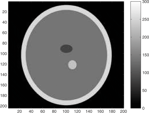
Figure 3. Original data set used in tests.

Figure 3. Original data set used in tests.

Figure 4. Projection data for 16, 32, 64 and 128 directions. The abscissa corresponds to p* for each direction and the ordinate to the d-th direction. The intensity scale is the same for all images.
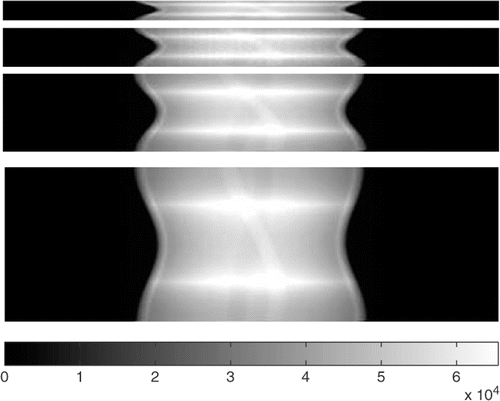
Figure 4. Projection data for 16, 32, 64 and 128 directions. The abscissa corresponds to p* for each direction and the ordinate to the d-th direction. The intensity scale is the same for all images.

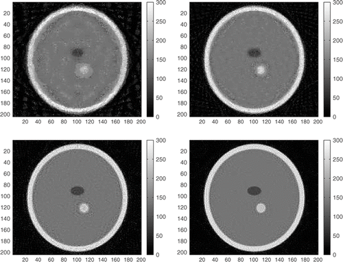
Figure 5. Results for the gΨ reconstruction method. D = 16, 32, 64 and 128.

Figure 5. Results for the gΨ reconstruction method. D = 16, 32, 64 and 128.

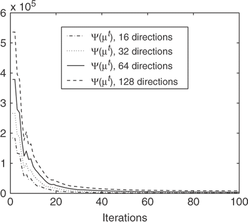
Figure 6. Objective function evolution for each case.

Figure 6. Objective function evolution for each case.

Figure 7. Projection data for PSNR 40 dB, 35 dB, 30 dB and 25 dB (128 directions). The abscissa corresponds to p* for each direction and the ordinate to the d-th direction.
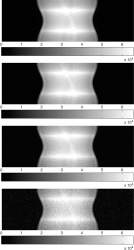
Figure 7. Projection data for PSNR 40 dB, 35 dB, 30 dB and 25 dB (128 directions). The abscissa corresponds to p* for each direction and the ordinate to the d-th direction.

Figure 8. Results for the gΨ reconstruction method from noise data with 128 directions for PSNR 40 dB, 35 dB, 30 dB and 25 dB (128 directions).
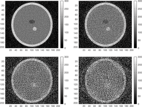
Figure 8. Results for the gΨ reconstruction method from noise data with 128 directions for PSNR 40 dB, 35 dB, 30 dB and 25 dB (128 directions).

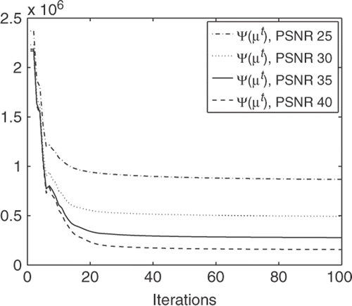
Figure 9. Objective function evolution for reconstruction with noise.

Figure 9. Objective function evolution for reconstruction with noise.

Figure 10. Projection data for different discretizations (1.1, 1.2, 1.3 and 1.4 spacings) and 128 directions. The abscissa corresponds to p* for each direction and the ordinate to the d-th direction.
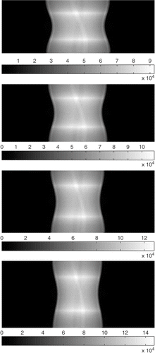
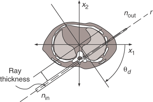
Figure 10. Projection data for different discretizations (1.1, 1.2, 1.3 and 1.4 spacings) and 128 directions. The abscissa corresponds to p* for each direction and the ordinate to the d-th direction.
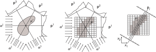
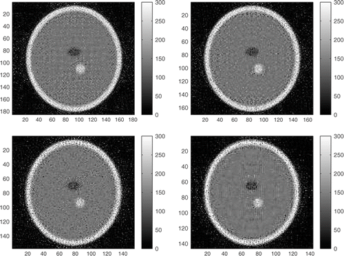
Figure 11. Results for the gΨ reconstruction method for different discretization in the reconstructed image (1.1, 1.2, 1.3 and 1.4 spacings, 128 directions).

Figure 11. Results for the gΨ reconstruction method for different discretization in the reconstructed image (1.1, 1.2, 1.3 and 1.4 spacings, 128 directions).

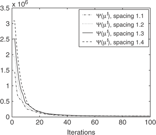
Figure 12. Objective function evolution for spacing 1.1, 1.2, 1.3 and 1.4.

Figure 12. Objective function evolution for spacing 1.1, 1.2, 1.3 and 1.4.

Reprints and Corporate Permissions

Please note: Selecting permissions does not provide access to the full text of the article, please see our help page How do I view content?

To request a reprint or corporate permissions for this article, please click on the relevant link below:

Academic Permissions

Please note: Selecting permissions does not provide access to the full text of the article, please see our help page How do I view content?

Obtain permissions instantly via Rightslink by clicking on the button below:

If you are unable to obtain permissions via Rightslink, please complete and submit this Permissions form. For more information, please visit our Permissions help page.