201
Views
4
CrossRef citations to date
0
Altmetric
Original Articles

Combining spatial support information and shape-based method for tomographic imaging inside a microwave cylindrical scanner

, &
Pages 19-34 | Received 15 Oct 2008, Accepted 28 Apr 2009, Published online: 23 Sep 2009

Figures & data

Figure 1. Picture and cross-section of the microwave scanner measurement set-up presently developed at Institut Fresnel.
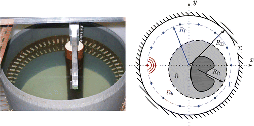
Figure 1. Picture and cross-section of the microwave scanner measurement set-up presently developed at Institut Fresnel.

Figure 2. (Available in colour online). Exact positioning of the three targets inside the tank in the synthetic configuration. Only the inner circular part of the tank with a radius of 10 cm is plotted.
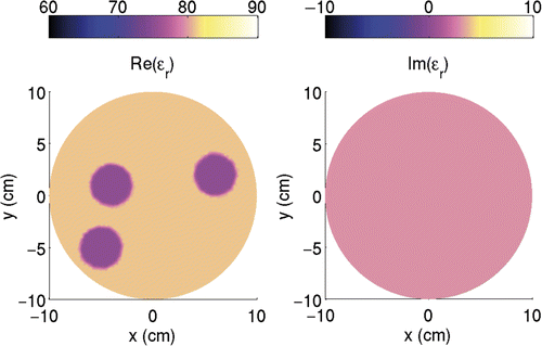
Figure 2. (Available in colour online). Exact positioning of the three targets inside the tank in the synthetic configuration. Only the inner circular part of the tank with a radius of 10 cm is plotted.

Figure 3. (Available in colour online). Real and imaginary permittivity profiles reconstructed at the end of the four iterative schemes. The results are obtained using the synthetic dataset starting with an initial estimate having the permittivity of the background. Only the inner circular part of the tank with a radius of 10 cm is plotted.
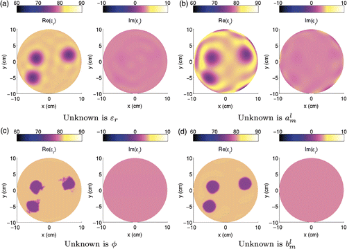
Figure 3. (Available in colour online). Real and imaginary permittivity profiles reconstructed at the end of the four iterative schemes. The results are obtained using the synthetic dataset starting with an initial estimate having the permittivity of the background. Only the inner circular part of the tank with a radius of 10 cm is plotted.

Figure 4. (Available in colour online). (a) Amplitude and (b) phase of the measured scattered field for each pair of emitter and receiver, when two tubes filled with a mixture of ethanol and water are positioned inside the water tank. The points which are too close to the emitting antenna are excluded.
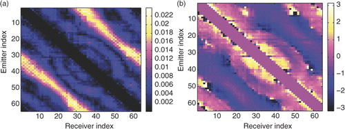
Figure 4. (Available in colour online). (a) Amplitude and (b) phase of the measured scattered field for each pair of emitter and receiver, when two tubes filled with a mixture of ethanol and water are positioned inside the water tank. The points which are too close to the emitting antenna are excluded.

Figure 5. (Available in colour online). Real and imaginary permittivity profiles reconstructed at the end of the four iterative schemes. The results are obtained using the experimental dataset, with an initial estimate having the permittivity of the background. Only the inner circular part of the tank with a radius of 10 cm is plotted.
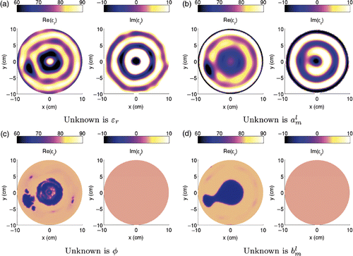
Figure 5. (Available in colour online). Real and imaginary permittivity profiles reconstructed at the end of the four iterative schemes. The results are obtained using the experimental dataset, with an initial estimate having the permittivity of the background. Only the inner circular part of the tank with a radius of 10 cm is plotted.

Figure 6. (Available in colour online). Real and imaginary permittivity profiles reconstructed at the end of the level-set function represented with Zernike polynomials. Several orders of Zernike polynomials are used to limit the number of unknown coefficients . The results are obtained using the experimental dataset, with an initial estimate having the permittivity of the background. Only the inner circular part of the tank with a radius 10 cm is plotted.
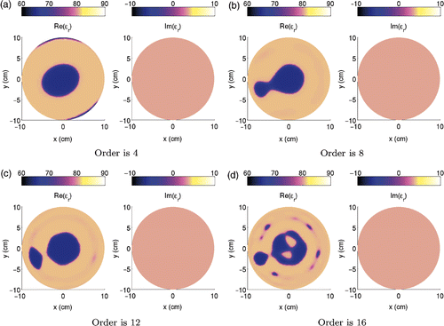
Figure 6. (Available in colour online). Real and imaginary permittivity profiles reconstructed at the end of the level-set function represented with Zernike polynomials. Several orders of Zernike polynomials are used to limit the number of unknown coefficients . The results are obtained using the experimental dataset, with an initial estimate having the permittivity of the background. Only the inner circular part of the tank with a radius 10 cm is plotted.

Figure 7. Evolution of the cost functional along the iterations. (a) The four schemes are compared. (b) The combination of the level-set function formalism and the Zernike polynomials representation is performed for various order of the Zernike polynomials. The dataset corresponds to the measured scattered field.
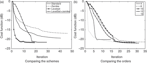
Figure 7. Evolution of the cost functional along the iterations. (a) The four schemes are compared. (b) The combination of the level-set function formalism and the Zernike polynomials representation is performed for various order of the Zernike polynomials. The dataset corresponds to the measured scattered field.

Reprints and Corporate Permissions

Please note: Selecting permissions does not provide access to the full text of the article, please see our help page How do I view content?

To request a reprint or corporate permissions for this article, please click on the relevant link below:

Academic Permissions

Please note: Selecting permissions does not provide access to the full text of the article, please see our help page How do I view content?

Obtain permissions instantly via Rightslink by clicking on the button below:

If you are unable to obtain permissions via Rightslink, please complete and submit this Permissions form. For more information, please visit our Permissions help page.