Solution of Cauchy problem to stationary heat conduction equation by modified method of elementary balances with interpolation of the solution in physical plane

Figures & data

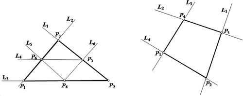
Figure 1. Arrangement of six mesh nodes of a triangular element or four nodes in a quadrilateral one.

Table 1. The numbers j₁ and j₂ of the straight line for the ith base function.

i	Triangle		Quadrilateral
	j1	j2	j1	j2
1	1	5	1	2
2	2	6	2	3
3	3	4	3	4
4	1	2	4	1
5	2	3
6	3	1

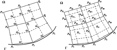
Figure 2. Four-node and nine-node elements of a quadrilateral mesh. The solid line denotes an interpolation mesh, while the broken one is for the balance mesh.

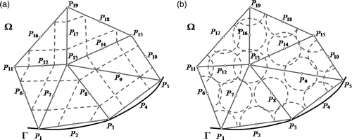
Figure 3. Six-node element of a triangular mesh; an example of control surface formulation (broken line): (a) polygonal region of balancing around node and (b) circular region of balancing.

Figure 4. Scheme of generation of system of equations in MCVM.

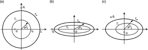
Figure 5. Region Ω: (a) circular ring, (b) elliptical ring, and (c) elliptical ring with displaced boundaries.

Figure 6. Boundary conditions for (a) direct problem (coefficient of heat exchange α on the boundary of the ring) and (b) inverse problem (temperature and density of heat flux on the outer boundary of the ring) in Example 1.

Figure 7. Boundary conditions for (a) direct problem (coefficient of heat exchange α on the boundary of the ring) and (b) inverse problem (temperature and density of heat flux on the outer boundary of the ring) in Example 2.

Figure 8. Boundary conditions for (a) direct problem (coefficient of heat exchange α on the boundary of the ring) and (b) inverse problem (temperature and density of heat flux on the outer boundary of the ring) in Example 3.

Figure 9. Boundary conditions for (a) direct problem (coefficient of heat exchange α on the boundary of the ring) and (b) inverse problem (temperature and density of heat flux on the outer boundary of the ring) in Example 4.

Table 2. Parameters of meshes of finite elements used in the numerical calculations.

	Triangular mesh elements			Quadrilateral mesh elements
Example	Number of inner nodes	Number of nodes on the boundary	Number of inner nodes	Number of nodes on the boundary	Number of inner nodes	Number of nodes on the boundary
1	700	200	400	800	200	900
2	3800	400	2000	3600	400	3800
3	1400	400	800	1600	400	1800
4	3800	400	2000	3600	400	3800
Note: The number of nodes on the inner boundary of the ring equals the number of nodes on the outer boundary.

Figure 10. Distribution (a) temperature and (b) density of heat flux on inner boundary of ring for undisturbed data, f = 5 in Example 1.

Figure 11. Distribution (a) temperature and (b) density of heat flux on inner boundary of ring for undisturbed data, f = 3 in Example 2.

Figure 12. Distributions (a) temperature and b) density of heat flux on inner boundary of ring for undisturbed data, f = 5 for triangular element and f = 3 for quadrilateral element in Example 3.

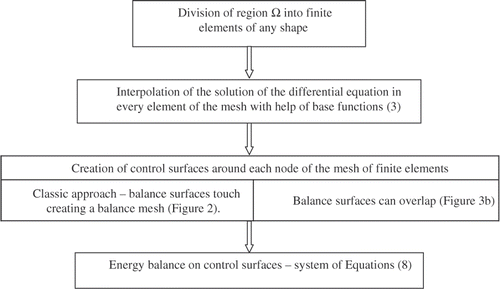
Figure 13. Distribution (a) temperature and (b) density of heat flux on inner boundary of ring for undisturbed data f = 3 in Example 4.

Table 3. Comparison of relative errors in the norm (17) for the temperature with respect to the problem type, the f parameter of the SVD algorithm and the number of base functions m serving for smoothing the disturbed boundary conditions in Example 1.

		Triangular mesh element					Quadrilateral mesh element
Type		The error, εmax (%)					The error, εmax (%)
m	f	0	0.5	1	5	10	0	0.5	1	5	10
The direct problem
		0.24	0.25	0.30	0.76	2.06	0.14	0.16	0.23	0.82	2.14
The inverse problem
	3	1.23	1.66	3.05	11.57	35.95	1.71	1.79	1.83	5.09	10.44
	5	0.7	18.18	30.22			0.33	6.35	10.63	54.85
	8	0.7	12.61	36.37			6.66
	10	0.7	26.31	32.97			6.66
	12	14.8	27.03	99.06			6.66
The inverse problem with smoothed boundary conditions
90	3	1.51	1.56	1.9	4.22	8.6	1.71	1.74	1.81	3.11	5.58
	5	1.12	14.15	24.3			0.33	8.12	13.26	42.55
	8	1.12	13.93	37.38			6.66
	10	1.12	14	31.28			6.66
	12	55.76	59.74	68.05	55.76	55.89	6.66
20	3	1.51	1.52	1.56	1.88	3.52	1.71	1.72	1.73	2.36	3.62
	5	1.13	3.37	6.02	24.61	46.72	0.33	7.49	11.35	35.56
	8	1.13	2.33	3.75	21.8	49.02	0.38	17	27.57
	10	1.13	1.96	3.33	27.81	35.59	0.38	20.68	23.94
12	55.76	55.8	55.8	59.82	65.29	0.38	48.08
4	3	2.9	2.9	2.9	2.9	3.33	2.74	2.74	2.74	2.87	3.46
	5	2.9	2.89	2.9	2.93	3.61	2.74	2.74	2.75	2.81	2.99
	8	2.9	2.89	2.91	2.92	3.08	2.74	2.74	2.74	2.82	2.75
	10	2.9	2.9	2.9	2.96	2.93	2.74	2.74	2.74	2.78	3
	12	55.83	55.82	55.81	55.95	55.79	2.74	2.74	2.74	2.82	3.12

Table 4. Comparison of relative errors in the norm (17) for the temperature with respect to the problem type, the f parameter of the SVD algorithm, and the number of base functions m serving for smoothing the disturbed boundary conditions in Example 2.

		Triangular mesh element					Quadrilateral mesh element
Type		The error, εmax (%)					The error, εmax (%)
m	f	0	0.5	1	5	10	0	0.5	1	5	10
The direct problem
		0.07	0.07	0.07	0.12	0.22	0.01	0.02	0.03	0.09	0.19
The inverse problem
	3	1.08	1.77	4.14	10.75	17.90	1.72	1.74	1.80	3.20	5.84
	5	1.15					0.34	5.15	20.48
The inverse problem with smoothed boundary conditions
90	3	1.51	1.56	1.9	4.22	8.6	1.71	1.74	1.81	3.11	5.58
	5	1.09	1.10	1.23	2.28	5.50	1.72	1.73	1.77	2.45	4.27
	8	1.74	11.95	11.24			0.34	13.69	13.35
20	3	1.10	1.12	1.16	2.07	4.06	1.73	1.74	1.75	1.97	3.09
	5	1.74	4.18	12.25			0.38	6.50	14.55
	8	1.74	6.16	14.81			0.38	6.83	17.76
4	3	3.55	3.55	3.55	3.61	3.60	3.54	3.54	3.54	3.61	3.60
	5	3.55	3.55	3.55	3.58	3.66	3.54	3.54	3.55	3.58	3.65

Table 5. Comparison of relative errors in the norm (17) for the temperature with respect to the problem type, the f parameter of the SVD algorithm, and the number of base functions m serving for smoothing the disturbed boundary conditions in Example 3.

		Triangular mesh element					Quadrilateral mesh element
Type		The error, εmax (%)					The error, εmax (%)
m	f	0	0.5	1	5	10	0	0.5	1	5	10
The direct problem
		0.10	0.09	0.10	0.27	0.30	0.02	0.03	0.07	0.23	0.30
The inverse problem
	3						0.65	0.69	0.83	2.81	4.96
	5	0.30	1.53	2.93	12.47	21.83	0.09	7.31
	8	0.18
The inverse problem with smoothed boundary conditions
90	3						0.65	0.71	0.75	1.91	3.97
	5	0.31	0.61	1.03	5.16		0.17
	8	1.13	4.22	7.71			5.67
20	3						0.88	0.88	0.90	1.41	2.37
	5	0.86	0.93	1.07	2.20	4.05	5.56	5.52	6.80	4.95
	8	2.90	2.69	3.34	6.14	5.22
4	3						6.76	6.76	6.78	6.67	6.97
	5	6.82	6.84	6.84	6.79	6.99	7.23	7.25	7.25	7.20	7.41
	8	6.89	6.88	6.92	6.78	6.73

Table 6. Comparison of relative errors in the norm (17) for the temperature with respect to the problem type, the f parameter of the SVD algorithm, and the number of base functions m serving for smoothing the disturbed boundary conditions in Example 4.

		Triangular mesh element					Quadrilateral mesh element
Type		The error, εmax (%)					The error, εmax (%)
m	f	0	0.5	1	5	10	0	0.5	1	5	10
The direct problem
		0.06	0.06	0.06	0.15	0.19	0.01	0.02	0.04	0.12	0.19
The inverse problem
	3	5.12	5.20	5.35	8.28		1.34	1.37	1.42	3.03	5.28
	5	0.32	3.59	8.69			0.12
	8	1.17					2.35
The inverse problem with smoothed boundary conditions
90	3	5.12	5.12	5.14	5.61	6.59	1.34	1.35	1.38	2.41	3.51
	5	0.33	0.70	1.22	7.41		0.12	9.48	8.51
	8	1.11					2.35
20	3	5.12	5.13	5.10	5.18	5.76	1.34	1.34	1.34	1.68	2.50
	5	0.34	0.71	1.38	5.16		0.59	1.20	3.66	9.74
	8	3.44
4	3	6.58	6.58	6.57	6.61	6.56	4.41	4.41	4.41	4.43	4.43
	5	4.91	4.91	4.91	4.91	4.98	5.82	5.82	5.81	5.80	5.92

Table 7. Comparison of relative errors in the norm (17) for the flux with respect to the problem type, the f parameter of the SVD algorithm and the number of base functions m serving for smoothing the disturbed boundary conditions in Example 1.

		Triangular mesh element					Quadrilateral mesh element
Type		The error, εmax (%)					The error, εmax (%)
m	f	0	0.5	1	5	10	0	0.5	1	5	10
The direct problem
		2.77	3.24	4.03	15.18	28.70	1.55	2.14	3.12	13.82	25.60
The inverse problem
	3	14.44	15.75	22.06	90.10		17.93	18.13	18.18	31.44	62.61
	5	6.40					8.02
	8	6.40
	10	6.40
The inverse problem with smoothed boundary conditions
90	3	14.49	14.71	15.26	20.63	47.92	17.93	18.04	18.20	22.71	33.49
	5	6.51					8.02
	8	6.51
	10	6.51
20	3	14.49	14.51	14.98	16.91	22.24	17.93	17.94	17.99	19.65	25.57
	5	6.79					8.02
	8	6.79	48.19				11.78
	10	6.79	40.01				11.78
4	3	22.61	22.61	22.61	22.68	23.61	22.50	22.50	22.50	22.92	24.84
5	22.61	22.61	22.61	23.00	24.88	22.50	22.50	22.51	22.68	23.44
	8	22.61	22.61	22.61	22.81	23.55	22.50	22.50	22.50	22.71	22.53
	10	22.61	22.62	22.61	22.73	22.65	22.50	22.50	22.50	22.59	23.10

Table 8. Comparison of relative errors in the norm (17) for the flux with respect to the problem type, the f parameter of the SVD algorithm, and the number of base functions m serving for smoothing the disturbed boundary conditions in Example 3.

		Triangular mesh element					Quadrilateral mesh element
Type		The error, εmax (%)					The error, εmax (%)
m	f	0	0.5	1	5	10	0	0.5	1	5	10
The direct problem
		0.58	0.63	0.78	2.81	5.69	0.07	0.27	0.51	2.54	5.37
The inverse problem
	3						17.31	17.29	17.57	27.17	34.05
	5	10.07	35.43				8.24
The inverse problem with smoothed boundary conditions
90	3						17.31	17.67	17.43	21.34	47.46
	5	9.88	16.02	24.55			12.23
20	3						17.61	17.57	17.79	21.54	26.26
	5	18.95	21.42	24.32	50.07
4	3						37.91	37.91	37.93	37.88	37.79
	5	40.48	40.50	40.51	40.50	40.39

Table 9. Comparison of relative errors in the norm (17) for the flux with respect to the problem type, the f parameter of the SVD algorithm, and the number of base functions m serving for smoothing the disturbed boundary conditions in Example 2.

		Triangular mesh element					Quadrilateral mesh element
Type		The error, εmax (%)					The error, εmax (%)
m	f	0	0.5	1	5	10	0	0.5	1	5	10
The direct problem
		0.59	0.68	0.84	2.62	5.39	0.12	0.30	0.56	2.58	5.20
The inverse problem
	3	24.28	30.99				30.71	30.72	30.82	33.02	39.72
	5						12.66
The inverse problem with smoothed boundary conditions
90	3	24.30	24.45	25.21	25.73	57.60	30.71	30.72	30.77	31.42	36.68
	5	66.69					12.66
20	3	24.32	24.37	24.53	31.67	48.62	30.72	30.74	30.75	30.86	34.52
	5	66.70					12.69
4	3	40.17	40.21	40.16	40.85	40.37	40.15	40.19	40.13	40.83	40.35
	5	40.17	40.18	40.19	40.35	39.77	40.15	40.16	40.17	40.33	39.74

Table 10. Comparison of relative errors in the norm (17) for the flux with respect to the problem type, the f parameter of the SVD algorithm, and the number of base functions m serving for smoothing the disturbed boundary conditions in Example 4.

		Triangular mesh element					Quadrilateral mesh element
Type		The error, εmax (%)					The error, εmax (%)
m	f	0	0.5	1	5	10	0	0.5	1	5	10
The direct problem
		0.53	0.59	0.86	2.61	5.26	0.11	0.25	0.59	2.58	5.13
The inverse problem
	3	53.53	53.53	53.50	53.78	54.68	27.38	27.38	27.44	31.23	30.03
	5	11.30					5.45
The inverse problem with smoothed boundary conditions
90	3	53.53	53.53	53.54	53.64	53.76	27.38	27.40	27.38	30.84	32.04
	5	11.30	18.79	29.49			5.48
20	3	53.53	53.53	53.54	53.56	53.52	27.38	27.38	27.49	28.01	29.67
	5	11.88	18.66	36.40			21.35	38.41
4	3	53.98	53.98	53.98	54.00	53.94	47.56	47.56	47.54	47.61	47.50