Figures & data
Figure 1. Semi-automatic localization of the outer and the inner surfaces of the thin soft tissue volume. The outer grid is depicted over the face (left). The inner grid is depicted over the skull with transperancy (right).
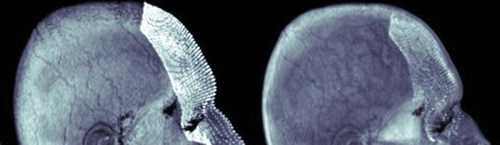
Figure 2. (a) The cameras and the force sensor probe positioned on a tripot. (b) The force sensor, the probe and the measurement device.
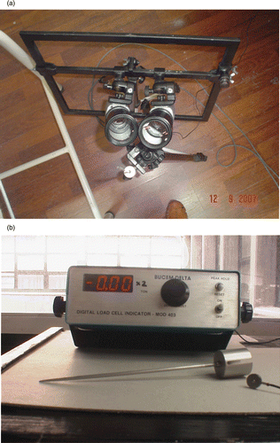
Figure 3. Calibration images.
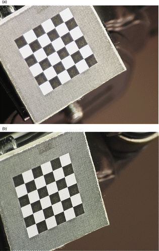
Figure 4. Stereo images collected when force is not applied (a and b) and when force is applied (c and d).
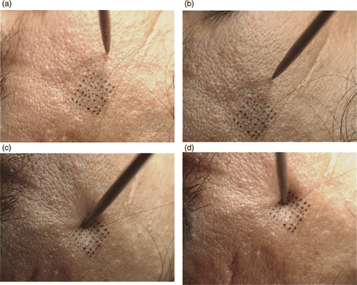
Figure 5. Marking on the face by the metal grid.
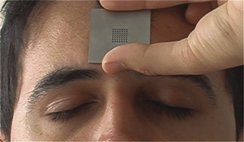
Figure 6. Graphical user interface of the programme, which is used to label the points on the surface, the contact point and the direction of the force.
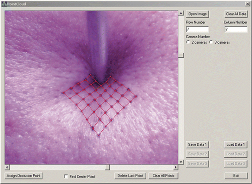
Figure 7. Position of the patient while a small force is applied on the forehead.
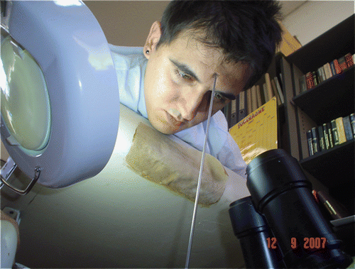
Figure 8. (Available in colour online) (a) 3D point cloud for the surface before (blue) and after (red) the force application. (b) Different views of the spline surfaces fit to the point cloud surfaces. Yellow is the initial surface (before force application) and red is the deformed surface (after force application). (c) The whole deformed surface obtained from the one-fourth. The smaller mesh (red dots) is the reconstructed shape. The whole deformed surface (the bigger mesh) is approximated by the symmetries of the reconstructed mesh.
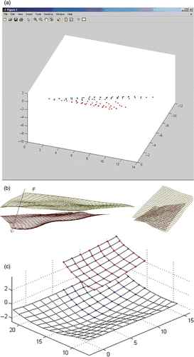
Figure 9. The actual initial surface (a) and the actual final surface (b) when 270 mN is applied on the forehead.
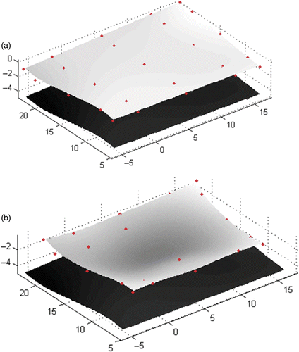
Figure 10. Force versus displacement plot where the slope is 60 N m−1.
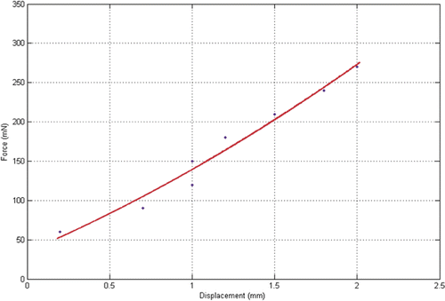
Figure 11. Shape of the skin volume outer surface at rest (a) when 300 mN (b) and 1000 mN (c) is applied in the direction pointed by the arrow. Red dots are the control points of the volume spline model.
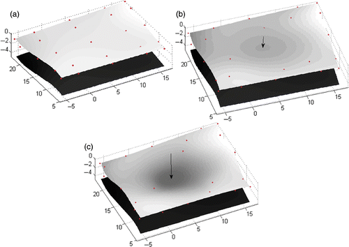
Figure 12. Marking on the face and the face MR data registered to the marked face region.
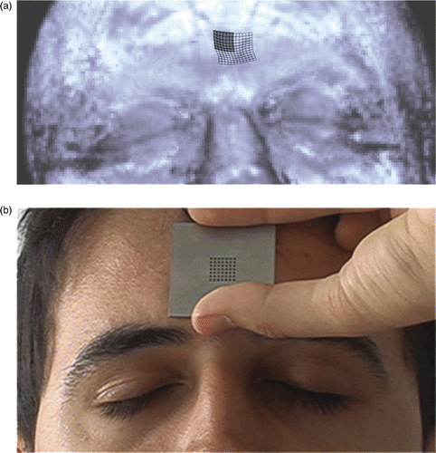
Figure 13. Forward and inverse solution steps.
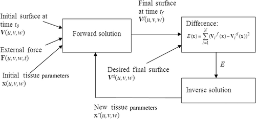
Figure 14. (a) The inital surface before the application of force, (b) the desired facial surface and (c) the result of the forward solution of the model when 1100 kg m−3, 50 N m−1, 24 Ns m−1 are used as mass density, stiffness and damping coefficients.
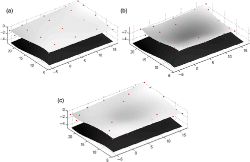
Table 1. Estimated parameter values for different initial values where the true values are 0.1 and 5 N m−1 for the horizontal and the vertical stiffness, respectively.
Figure 15. The desired surface obtained during the experiment (a) and the final surface obtained by the parameter values estimated after the inverse solution (b) when the objective function value becomes 9 × 10⁻⁶ at the end of optimization iterations.
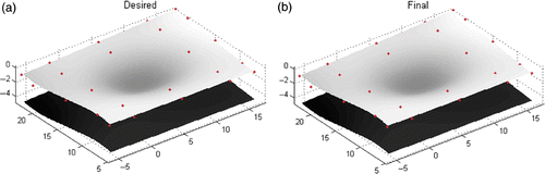
Figure 16. (Available in colour online). (a) Facial muscles, namely corrugator (1, 2), frontalis (3, 4), zygomatic major (5, 6), caninus (7, 8), risorius (9, 10) and triangularis (11, 12), are shown over the segmented skull. (b) Muscles are shown as linear vectors emerging from the origin points (red crosses) towards the instertion points (green circles) on the inner soft tissue layer. (c) The muscle vectors are depicted inside the inner soft tissue layer.
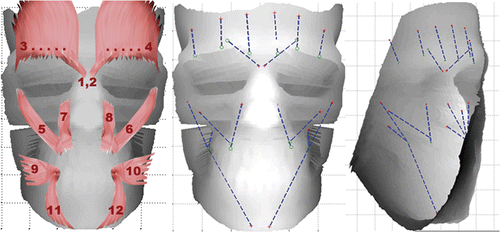
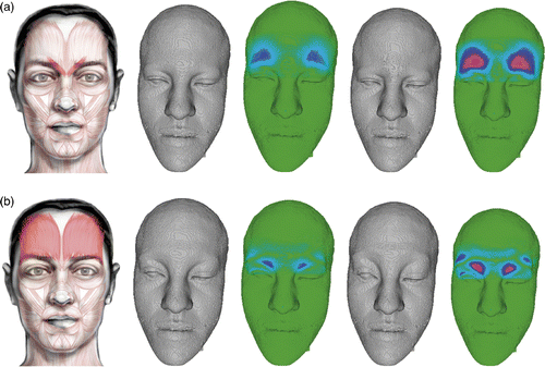
Figure 17. (Available in colour online). Facial expression simulation by the contraction of (a) frontalis and (b) corrugator muscles. For each muscle, two different degrees of contraction (first less, then more) are given. The difference between the resting face model and the animated face model is also depicted in colour scale. Green–ındifferent, blue–moderately different and red–most different.