1,111
Views
32
CrossRef citations to date
0
Altmetric
Original Articles

A numerical method for solving the inverse heat conduction problem without initial value

, , &
Pages 655-671 | Received 24 Nov 2008, Accepted 08 Feb 2010, Published online: 19 Apr 2010

Figures & data

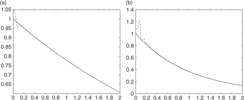
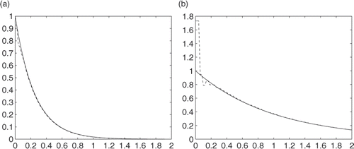
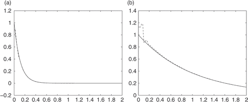
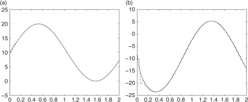
Figure 1. Schematic representation of K = 0.5, without noise: (a) u(0, t) and (b) .

Figure 1. Schematic representation of K = 0.5, without noise: (a) u(0, t) and (b) .

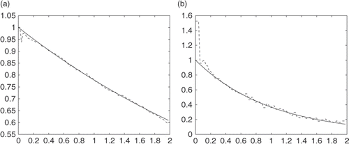
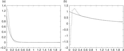
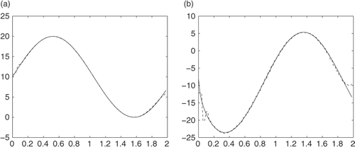
Figure 2. Schematic representation of K = 0.5, with 0.5% random noise: (a) u(0, t) and (b) .

Figure 2. Schematic representation of K = 0.5, with 0.5% random noise: (a) u(0, t) and (b) .

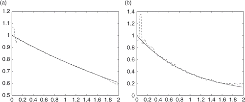
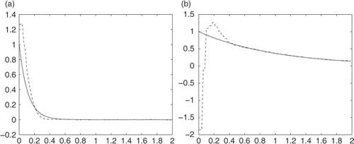
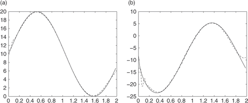
Figure 3. Schematic representation of K = 0.5, with 1% random noise: (a) u(0, t) and (b) .

Figure 3. Schematic representation of K = 0.5, with 1% random noise: (a) u(0, t) and (b) .

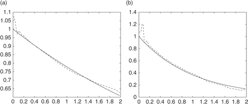
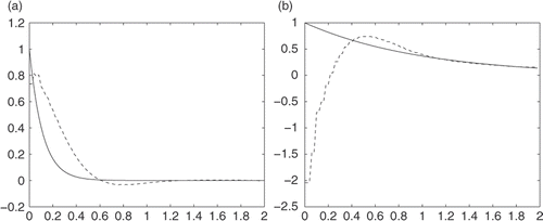
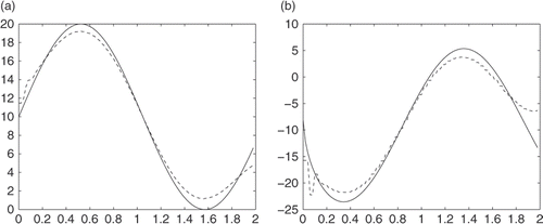
Figure 4. Schematic representation of K = 0.5, with 3% random noise: (a) u(0, t) and (b) .

Figure 4. Schematic representation of K = 0.5, with 3% random noise: (a) u(0, t) and (b) .

Figure 5. Graph of K = 2, without noise: (a) u(0, t) and (b) .

Figure 5. Graph of K = 2, without noise: (a) u(0, t) and (b) .

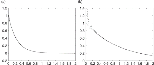
Figure 6. Graph of K = 2, with 0.5% random noise: (a) u(0, t) and (b) .

Figure 6. Graph of K = 2, with 0.5% random noise: (a) u(0, t) and (b) .

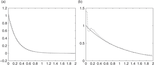
Figure 7. Graph of K = 2, with 1% random noise: (a) u(0, t) and (b) .

Figure 7. Graph of K = 2, with 1% random noise: (a) u(0, t) and (b) .

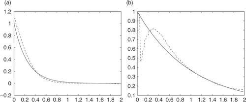
Figure 8. Graph of K = 2, with 3% random noise: (a) u(0, t) and (b) .

Figure 8. Graph of K = 2, with 3% random noise: (a) u(0, t) and (b) .

Figure 9. Graph of K = 3, without noise: (a) u(0, t) and (b) .

Figure 9. Graph of K = 3, without noise: (a) u(0, t) and (b) .

Figure 10. Graph of K = 3, with 0.5% random noise: (a) u(0, t) and (b) .

Figure 10. Graph of K = 3, with 0.5% random noise: (a) u(0, t) and (b) .

Figure 11. Graph of K = 3, with 1% random noise: (a) u(0, t) and (b) .

Figure 11. Graph of K = 3, with 1% random noise: (a) u(0, t) and (b) .

Figure 12. Graph of K = 3, with 3% random noise: (a) u(0, t) and (b) .

Figure 12. Graph of K = 3, with 3% random noise: (a) u(0, t) and (b) .

Table 1. Absolute errors with different noise level and K.

Figure 13. Graph of (a) u(0, t) and (b) , without random noise.

Figure 13. Graph of (a) u(0, t) and (b) , without random noise.

Figure 14. Graph of (a) u(0, t) and (b) , with 0.5% random noise.

Figure 14. Graph of (a) u(0, t) and (b) , with 0.5% random noise.

Figure 15. Graph of (a) u(0, t) and (b) , with 1% random noise.

Figure 15. Graph of (a) u(0, t) and (b) , with 1% random noise.

Figure 16. Graph of (a) u(0, t) and (b) , with 3% random noise.

Figure 16. Graph of (a) u(0, t) and (b) , with 3% random noise.

Table 2. Absolute errors with different noise level.

Reprints and Corporate Permissions

Please note: Selecting permissions does not provide access to the full text of the article, please see our help page How do I view content?

To request a reprint or corporate permissions for this article, please click on the relevant link below:

Academic Permissions

Please note: Selecting permissions does not provide access to the full text of the article, please see our help page How do I view content?

Obtain permissions instantly via Rightslink by clicking on the button below:

If you are unable to obtain permissions via Rightslink, please complete and submit this Permissions form. For more information, please visit our Permissions help page.