404
Views
25
CrossRef citations to date
0
Altmetric
Original Articles

Numerical approximation of the one-dimensional inverse Cauchy–Stefan problem using a method of fundamental solutions

, &
Pages 659-677 | Received 16 Mar 2011, Accepted 26 Mar 2011, Published online: 13 Jul 2011

Figures & data

Figure 1. General representation of the domain D and boundary Γ = ΓU ∪ ΓS, with unspecified initial and boundary conditions (·····) on ΓU, collocation points () on ΓS and source points (- - -) placed on external to the domain D.
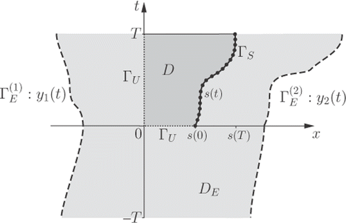
Figure 1. General representation of the domain D and boundary Γ = ΓU ∪ ΓS, with unspecified initial and boundary conditions (·····) on ΓU, collocation points () on ΓS and source points (- - -) placed on external to the domain D.

Figure 2. Particularization of for s(t) given by Equation (17) in Example 1.
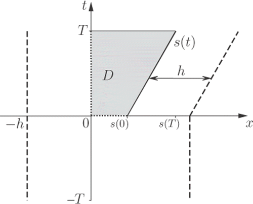
Figure 2. Particularization of Figure 1 for s(t) given by Equation (17) in Example 1.

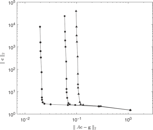
Figure 3. L-curve plots for δ = 1% (—–), δ = 3% () and δ = 5% () when M = 30 in (12), for Example 1.

Figure 3. L-curve plots for δ = 1% (—–), δ = 3% () and δ = 5% () when M = 30 in (12), for Example 1.

Figure 4. The exact solutions (—–) and MFS approximations for: (a) u(0, t), (b) ux(0, t) and (c) u(x, 0). All MFS approximations have been generated for noise levels δ = 1% (•) with λ = 10−6, δ = 3% (▪) with λ = 10−5 and δ = 5% (▴) with λ = 10−5, and obtained with h = 2, and M = 30, for Example 1.
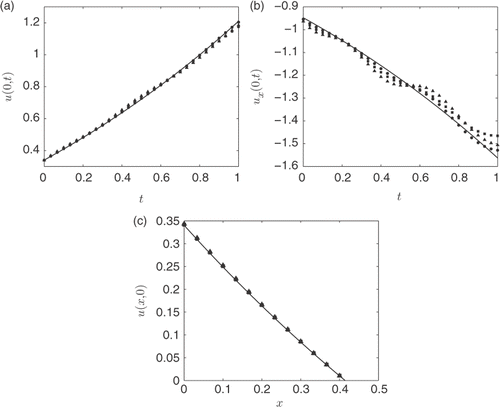
Figure 4. The exact solutions (—–) and MFS approximations for: (a) u(0, t), (b) ux(0, t) and (c) u(x, 0). All MFS approximations have been generated for noise levels δ = 1% (•) with λ = 10−6, δ = 3% (▪) with λ = 10−5 and δ = 5% (▴) with λ = 10−5, and obtained with h = 2, and M = 30, for Example 1.

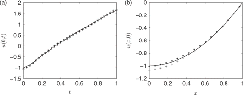
Figure 5. Plots of the exact solution (—–) and the best (*) and least (+) accurate MFS approximations from 10 different sets of noisy data with noise level δ = 5% for (a) u(0, t) and (b) u(x, 0). Both plots are obtained with h = 2, M = 30 and λ = 10−5, for Example 1.
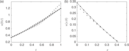
Figure 5. Plots of the exact solution (—–) and the best (*) and least (+) accurate MFS approximations from 10 different sets of noisy data with noise level δ = 5% for (a) u(0, t) and (b) u(x, 0). Both plots are obtained with h = 2, M = 30 and λ = 10−5, for Example 1.

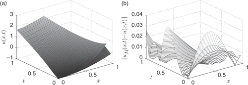
Figure 6. (a) The exact solution u(x, t) for all (x, t) ∈ D and (b) the absolute error for all (x, t) ∈ D for noise level δ = 5%, obtained with h = 2, λ = 10−5, M = 30, for Example 1.
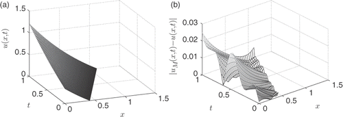
Figure 6. (a) The exact solution u(x, t) for all (x, t) ∈ D and (b) the absolute error for all (x, t) ∈ D for noise level δ = 5%, obtained with h = 2, λ = 10−5, M = 30, for Example 1.

Figure 7. Plots of the absolute error for all (x, t) ∈ D for noise level δ = 5% obtained with h = 2.5, λ = 10−6 and (a) M = 30 and (b) M = 16, for Example 1.

Figure 7. Plots of the absolute error for all (x, t) ∈ D for noise level δ = 5% obtained with h = 2.5, λ = 10−6 and (a) M = 30 and (b) M = 16, for Example 1.

Figure 8. Particularization of for s(t) given by Equation (25) in Example 2.
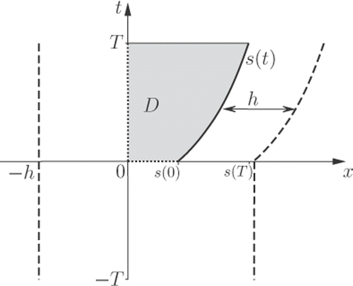
Figure 8. Particularization of Figure 1 for s(t) given by Equation (25) in Example 2.

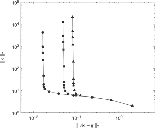
Figure 9. L-curve plots for δ = 1% (), δ = 3% () and δ = 5% () when M = 30, for Example 2.

Figure 9. L-curve plots for δ = 1% (), δ = 3% () and δ = 5% () when M = 30, for Example 2.

Figure 10. The exact solutions (—–) and MFS approximations for: (a) u(0, t), (b) ux(0, t) and (c) u(x, 0). All MFS approximations have been generated for noise levels δ = 1% (•) with λ = 10−6, δ = 3% (▪) with λ = 10−5 and δ = 5% (▴) with λ = 10−5, and obtained with h = 2, and M = 30, for Example 2.
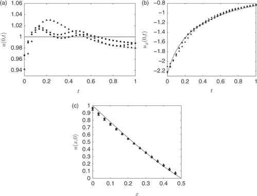
Figure 10. The exact solutions (—–) and MFS approximations for: (a) u(0, t), (b) ux(0, t) and (c) u(x, 0). All MFS approximations have been generated for noise levels δ = 1% (•) with λ = 10−6, δ = 3% (▪) with λ = 10−5 and δ = 5% (▴) with λ = 10−5, and obtained with h = 2, and M = 30, for Example 2.

Figure 11. Plots of the exact solution (—–) and the best (*) and least (+) accurate MFS approximations from 10 different sets of noisy data with noise level δ = 5% for (a) u(0, t) and (b) u(x, 0). Both plots are obtained with h = 2, M = 30 and λ = 10−4, for Example 2.
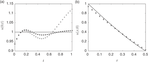
Figure 11. Plots of the exact solution (—–) and the best (*) and least (+) accurate MFS approximations from 10 different sets of noisy data with noise level δ = 5% for (a) u(0, t) and (b) u(x, 0). Both plots are obtained with h = 2, M = 30 and λ = 10−4, for Example 2.

Figure 12. (a) The exact solution u(x, t) for all and (b) the absolute error for all (x, t) ∈ D for noise level δ = 5%, obtained with h = 2, λ = 10−5, M = 30, for Example 2.
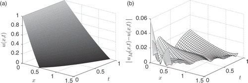
Figure 12. (a) The exact solution u(x, t) for all and (b) the absolute error for all (x, t) ∈ D for noise level δ = 5%, obtained with h = 2, λ = 10−5, M = 30, for Example 2.

Figure 13. Particularization of for s(t) given by Equation (32) in Example 3.
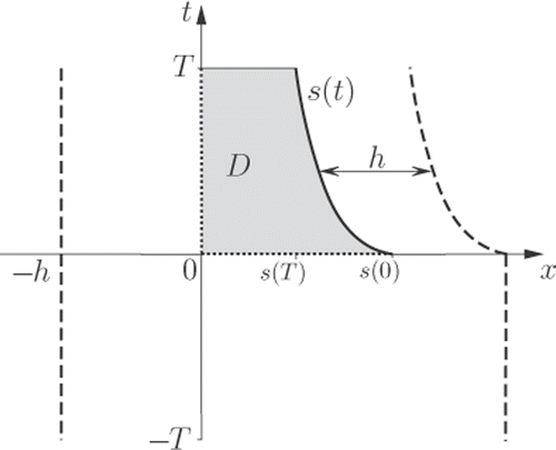
Figure 13. Particularization of Figure 1 for s(t) given by Equation (32) in Example 3.

Figure 14. (a) The exact solution u(0, t) (—–) and the MFS approximation, and (b) the exact solution u(x, 0) (—–) and the MFS approximation. Both plots are obtained with λ = 10−8, h = 2 and M = 30, for Example 3.
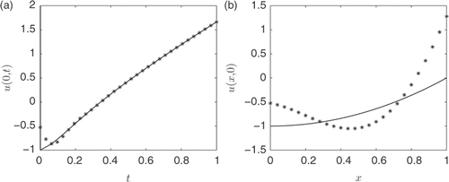
Figure 14. (a) The exact solution u(0, t) (—–) and the MFS approximation, and (b) the exact solution u(x, 0) (—–) and the MFS approximation. Both plots are obtained with λ = 10−8, h = 2 and M = 30, for Example 3.

Figure 15. L-curve plots with the singularity removed for δ = 1% (), δ = 3% () and δ = 5% () when M = 30, for Example 3.

Figure 15. L-curve plots with the singularity removed for δ = 1% (), δ = 3% () and δ = 5% () when M = 30, for Example 3.

Figure 16. The exact solutions (—–) and MFS approximations with singularity removed for: (a) u(0, t), (b) ux(0, t) and (c) u(x, 0). All MFS approximations have been generated for noise levels δ = 1% (•) with λ = 10−6, δ = 3% (▪) with λ = 10−5 and δ = 5% (▴) with λ = 10−5, and obtained with h = 2, and M = 30, for Example 3.
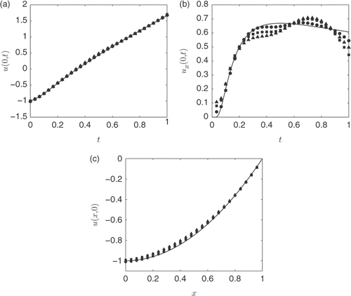
Figure 16. The exact solutions (—–) and MFS approximations with singularity removed for: (a) u(0, t), (b) ux(0, t) and (c) u(x, 0). All MFS approximations have been generated for noise levels δ = 1% (•) with λ = 10−6, δ = 3% (▪) with λ = 10−5 and δ = 5% (▴) with λ = 10−5, and obtained with h = 2, and M = 30, for Example 3.
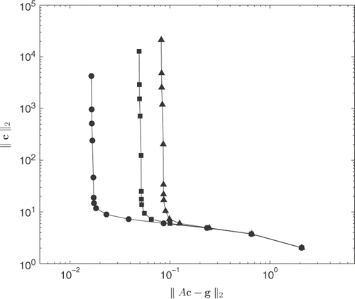
Figure 17. Plots of the exact solution (—–) and the best (*) and least (+) accurate MFS approximations from 10 different sets of noisy data with noise level δ = 5% for (a) u(0, t) and (b) u(x, 0). Both plots are obtained with the singularity removed, h = 2, M = 30 and λ = 10−4, for Example 3.

Figure 17. Plots of the exact solution (—–) and the best (*) and least (+) accurate MFS approximations from 10 different sets of noisy data with noise level δ = 5% for (a) u(0, t) and (b) u(x, 0). Both plots are obtained with the singularity removed, h = 2, M = 30 and λ = 10−4, for Example 3.

Figure 18. (a) The exact solution u(x, t) for all and (b) the absolute error for all (x, t) ∈ D for noise level δ = 5%, obtained with the singularity removed, h = 2, λ = 10−5, M = 30, for Example 3.

Figure 18. (a) The exact solution u(x, t) for all and (b) the absolute error for all (x, t) ∈ D for noise level δ = 5%, obtained with the singularity removed, h = 2, λ = 10−5, M = 30, for Example 3.

Reprints and Corporate Permissions

Please note: Selecting permissions does not provide access to the full text of the article, please see our help page How do I view content?

To request a reprint or corporate permissions for this article, please click on the relevant link below:

Academic Permissions

Please note: Selecting permissions does not provide access to the full text of the article, please see our help page How do I view content?

Obtain permissions instantly via Rightslink by clicking on the button below:

If you are unable to obtain permissions via Rightslink, please complete and submit this Permissions form. For more information, please visit our Permissions help page.