Source characterization of atmospheric releases using stochastic search and regularized gradient optimization

Figures & data

Table 1. Salient features of various inversion techniques used to solve atmospheric source characterization problems.

Ref.	Model parameters (m)	Forward model (A)	Inversion technique	Validation procedure	Application	Performance
10	Qs	Steady laminar incompressible Navier-Stokes solver + ADE	Adjoint method	Synthetic data without noise	Contamination dispersion
16	xs, ys, zs, Qs, us, θs, δs	Gaussian puff	GA	Synthetic data without noise	Atmospheric source inversion
17	xs, ys, Qs	GPM	Detector footprint method	Synthetic data with and without noise	Atmospheric source inversion
8	xs, ys, zs, Qs	FEM3MP – 3D	Bayesian inference + MCMC	Synthetic and field data	Atmospheric source inversion	(1) 2560 forward runs (2) Total computation time: over 12 h on 1024 2.4 GHz Xeon processors
11	zs, ts	Chemistry transport model – POLAIR 3D	Adjoint method		Reconstruction of Chernobyl accident source term
18	xs, ys, Qs, us, θs, stability class	GPM	GA	Synthetic data without noise	Atmospheric source inversion	(1) 2000 generations meteorological parameters (2) 10,000 generations for xs, ys, Qs, θs & stability
12	fj,m, sOH, sstea, c0	Global atmospheric CTM	Adjoint method	Field data	Global-scale sources & sinks of methane
19	xs, ys, zs, Qs	GPM	Expectation maximization	Synthetic data without noise	Atmospheric source inversion
20	xs, ys, Qs, θs	Gaussian puff	GA + simplex optimization	Synthetic data without noise		(1) 1200 chromosomes (2) 100 GA iterations
21	Qs	Langevin model	Quasi-Newton and SA	Field data	Atmospheric source inversion	(1) 65 quasi-Newton iterations (2) 1575 SA iterations
9	xs, ys, zs, Qs, us, θs	GPM	Bayesian inference + MCMC	Field data	Atmospheric source inversion	50,000 MCMC evaluations
13	Kxx, u*, L, z0	2D ADE	Levenberg–Marquardt method	Field data	Identification of atmospheric boundary layer parameters
22	xs, ys, zs, Qs	GPM	SA	Field data	atmospheric ethane used to locate ground-level sources	4×10^6 iterations
Note: ts – temporal release profile, fj, m – integrated surface emission over region j & month m, sOH – parametrization for chemical removal of methane with hydroxyl radical, sstea – stratospheric methane loss, c0 – global mean methane concentration, Kxx – longitudinal turbulent diffusivity, u* – friction velocity, L – Monin-Obukhov length, z0 – aerodynamic surface roughness, CTM – chemistry transport model, GPM – Gaussian plume model, SA – simulated annealing, ADE – advection–diffusion equation, GA – genetic algorithm.

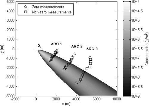
Figure 1. Schematic depicting the sensor positioning and the number of non-zero (□) and zero (○) measurements recorded for TCTE on 19 October. Also shown is the plume spread predicted by the GPM for true source parameters (m_t). ‘S_t’ is the true source location.

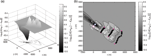
Figure 2. (a) Surface of the misfit functional for TCTE, (b) 2D contour of the misfit functional for TCTE data with the true (S_t) and predicted (S_p) source locations.

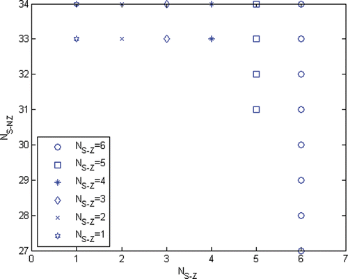
Figure 3. The number of zero (N_S−Z) and non-zero (N_S−NZ) measurements that should be satisfied to obtain initial iterates in the C-C-D region for TCTE. The details of this figure are highly problem-dependent. They also depend on the plume spread parameters chosen.

Table 2. Computed inversion model parameters for TCTE.

Model parameters	xS (m)	yS (m)	zS (m)	QS/uS (gm^−1)	θS (degrees)	NS
mt	0	0	115	0.64	308.57	–
mSTOCH	−650.81	736.72	3.08	0.73	297.22	37
mSTOCH*max(Ns)	91.05	−21.44	85.97	0.86	294.63	39
mSTOCH+GD	−339.78	73.6	193.42	1.06	291.73	34

Table 3. Comparison of the predicted concentrations from Newton's method with Copenhagen data (12 : 13 h–12 : 33 h on 19 October 1978) and 16.

Position	Sensor x-coordinate (m)	Sensor y-coordinate (m)	Observed concentration (ng m^−3)	Predicted concentration 16 (ng m^−3)	Predicted concentration from this work (ng m^−3)
9	1398	−1312	0	721	0
10	1404	−1214	0	135	28
11	1492	−1131	186	2271	259.4
12	1516	−1044	614	3266	896
13	1582	−964	1816	4478	2672
14	1592	−884	5455	5105	4642.9
15	1602	−798	7016	5727	6682.1
16	1703	−767	6770	5582	7161.6
17	1766	−681	5472	5077	5860.7
18	1800	−593	3806	4067	3523.4
19	1877	−485	1114	2842	1053.1
20	1921	−405	919	1969	320.4
21	2067	−371	77	1902	101.6
22	2061	−284	0	1001	22.5
23	2055	−180	0	463	0
11	2818	−2134	0	1400	53.3
12	2920	−1987	107	1579	295.3
13	3002	−1830	840	2635	1022.3
14	3075	−1704	1478	2691	2029.3
15	3204	−1629	3133	2580	2797.2
17	3380	−1367	2563	2249	2627.3
18	3448	−1231	2225	2033	1614.8
19	3518	−1093	538	1282	722.2
20	3558	−919	0	1050	194.8
21	3729	−787	0	361	33.4
22	3837	−550	0	121	0
9	4027	−3616	0	306	0
10	4283	−3447	18	788	0
11	4390	−3277	21	1087	12.4
12	4459	−3010	85	1117	97.6
13	4572	−2795	800	1552	396.8
14	4668	−2514	1502	1236	1180.5
15	4824	−2260	2035	1297	1762.0
16	5029	−2108	1112	1063	1476.7
17	5286	−1939	434	778	761.8
18	5378	−1570	53	124	129.9
19	5395	−1399	0	49	42.1
20	5375	−1139	0	109	0
21	5323	−913	0	47	0

Figure 4. Convergence of Newton's method for TCTE.

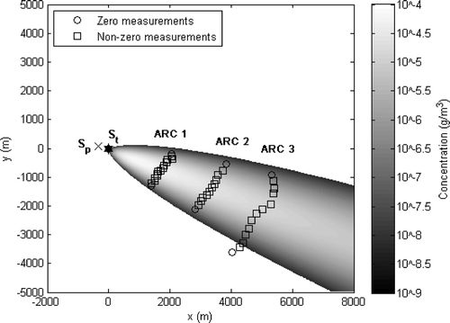
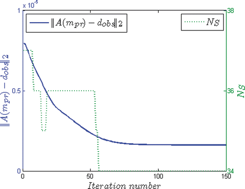
Figure 5. Plume spread predicted by model parameters from inversion. The squares (□) and the circles (○) represent sensors that recorded non-zero and zero measurements. ‘S_t’ (hexagon – ☆) is the true source location in, and ‘S_p’ (cross – ×) the location predicted by Newton's method.

Table 4. Computed inversion model parameters for TCTE using the dataset between 12 : 13 h and 12 : 33 h.

Model parameters	xS (m)	yS (m)	zS (m)	qS/uS (gm^−1)	θS (degrees)	NS
mt	0	0	115	0.64	308.57	–
mSTOCH+GD	64.001	2.58	181.49	1.11	295.11	32

Table 5. Performance of the various original QMC point-sets with SR1.

Point-sets	NS ≥ 37	NS ≥ 38	NS ≥ 39
E(MC)	12,633	82,102	25,000,000
O-Halton	6521	50,081	6666,989
O-Hammersley	678	17,730	4903,807
O-Sobol	1649	18,761	437,165
O-SplNie	24,377****	97,632****	1150,264
O-NieXing	10,040	159,266****	4434,687

Table 6. Performance of the various scrambled QMC point-sets with SR1.

Point-sets	NS ≥ 37	NS ≥ 38	NS ≥ 39
E(MC)	12,633	82,102	25,000,000
S-Halton	797	43,565	1740,461
S-Hammersley	2047	9250	–
S-Sobol	1230	23,758	1213,246
S-SplNie	29,265****	49,313	–
S-NieXing	6087	6087	2414,141

Table 7. Performance of the various original QMC point-sets with SR3.

Point-sets (NS−NZ = 34)	NS−Z ≥ 5	NS−Z ≥ 4	NS−Z ≥ 3	NS−Z ≥ 2	NS−Z ≥ 1
E(MC)	25,000,000	114,943	32,342	12,533	9371
O-Halton	6666,989	50,081	50,081****	50,081****	50,081****
O-Hammersley	5258,175	–	4010	678	90
O-Sobol	437,165	18,761	1649	1649	1649
O-SplNie	1150,264	97,632	81,072****	10,224	10,224****
O-NieXing	–	171,000****	22,536	2240	2240

Table 8. Performance of the various scrambled QMC point-sets with SR3.

Point-sets (NS−NZ = 34)	NS−Z ≥ 5	NS−Z ≥ 4	NS−Z ≥ 3	NS−Z ≥ 2	NS−Z ≥ 1
E(MC)	25,000,000	114,943	32,342	12,533	9371
S-Halton	18,025,133	188,933****	19,841	10,961	10,961
S-Hammersley	–	–	–	262	262
S-Sobol	–	23,758	1230	1230	1230
S-SplNie	–	49,313	29,265	10,609	9473****
S-NieXing	2414,141	6087	6087	4651	4651