921
Views
7
CrossRef citations to date
0
Altmetric
Original Articles

Denoising point cloud

, &
Pages 287-298 | Received 19 Jan 2010, Accepted 01 Jul 2011, Published online: 08 Aug 2011

Figures & data

Figure 1. Density function of point's shifts using Gaussian smoothing. For (a)–(d) eigenvalue follows uniform distribution and for (e)–(h) eigenvalue follows norm distribution: (a), (e)  = 0.5,  = 2. (b), (f)  = 0.2,  = 2. (c), (g)  = 0.2,  = 5. (d), (h)  = 0.2,  = 10.
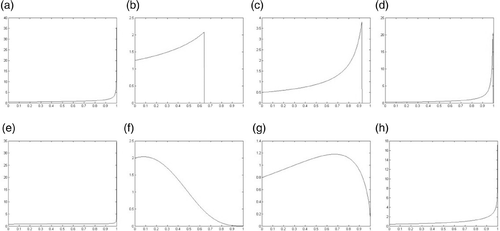
Figure 1. Density function of point's shifts using Gaussian smoothing. For (a)–(d) eigenvalue follows uniform distribution and for (e)–(h) eigenvalue follows norm distribution: (a), (e)  = 0.5,  = 2. (b), (f)  = 0.2,  = 2. (c), (g)  = 0.2,  = 5. (d), (h)  = 0.2,  = 10.

Figure 2. Density function of point's shifts using the λ/μ method. For (a)–(d) eigenvalue follows uniform distribution and for (e)–(h) eigenvalue follows norm distribution. (a), (e)  = 0.5,  = −0.51,  = 1. (b), (f)  = 0.2,  = −0.21,  = 1. (c), (g)  = 0.2,  = −0.21,  = 5. (d), (h)  = 0.2,  = −0.21,  = 10.
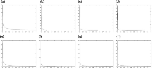
Figure 2. Density function of point's shifts using the λ/μ method. For (a)–(d) eigenvalue follows uniform distribution and for (e)–(h) eigenvalue follows norm distribution. (a), (e)  = 0.5,  = −0.51,  = 1. (b), (f)  = 0.2,  = −0.21,  = 1. (c), (g)  = 0.2,  = −0.21,  = 5. (d), (h)  = 0.2,  = −0.21,  = 10.

Figure 3. Denoising 2D noisy data taken from two concentric circles of radii 0.9 and 1.0. The noisy circles are illustrated with black points in (a)–(d). (a) and (b) show the point set after smoothing using λ/μ and LOP, respectively. (c) and (d) show the point set after 1 and 2 iterations using our method. In (e) and (f), green points denote the results of LOP, blue points denote the results using λ/μ and red points show the denoising point set using our method. In (a) and (e), a few remaining floating points still exist and three methods obtain similar results which are robust to noise. Moreover, the shrinkage effect is insignificant for three methods.

Figure 3. Denoising 2D noisy data taken from two concentric circles of radii 0.9 and 1.0. The noisy circles are illustrated with black points in (a)–(d). (a) and (b) show the point set after smoothing using λ/μ and LOP, respectively. (c) and (d) show the point set after 1 and 2 iterations using our method. In (e) and (f), green points denote the results of LOP, blue points denote the results using λ/μ and red points show the denoising point set using our method. In (a) and (e), a few remaining floating points still exist and three methods obtain similar results which are robust to noise. Moreover, the shrinkage effect is insignificant for three methods.

Figure 4. Denoising noisy data taken from two osculatory cylinders: (a) two noisy osculatory cylinders, (b) the result after one time's iteration using our method, (c) point set after three iterations using our method, (d) the result of LOP, (e) the combination results of our method and LOP and (f) our result and original point set. Our method shows more robust.
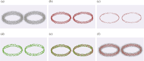
Figure 4. Denoising noisy data taken from two osculatory cylinders: (a) two noisy osculatory cylinders, (b) the result after one time's iteration using our method, (c) point set after three iterations using our method, (d) the result of LOP, (e) the combination results of our method and LOP and (f) our result and original point set. Our method shows more robust.

Figure 5. Example of denoising a complex point set: (a) the original 3D mesh model of a human face, (b) 3D mesh model after smoothing using λ/μ, (c) 3D mesh model after smoothing using LOP and (d) 3D mesh model after denoising using our method. (e), (f), (g) and (h) are the local magnified regions of (a), (b), (c) and (d), respectively.
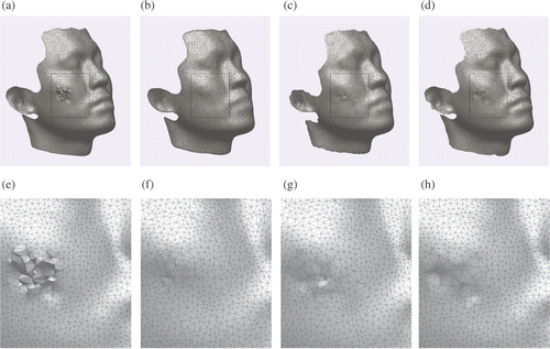
Figure 5. Example of denoising a complex point set: (a) the original 3D mesh model of a human face, (b) 3D mesh model after smoothing using λ/μ, (c) 3D mesh model after smoothing using LOP and (d) 3D mesh model after denoising using our method. (e), (f), (g) and (h) are the local magnified regions of (a), (b), (c) and (d), respectively.

Figure 6. Raw data set denoising example: (a) a noisy point set, (b) point set after smoothing using λ/μ method and (c) clean data after denoising using our method. (d), (e) and (f) are the local point sets which are corresponding to (a), (b) and (c).
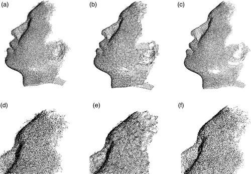
Figure 6. Raw data set denoising example: (a) a noisy point set, (b) point set after smoothing using λ/μ method and (c) clean data after denoising using our method. (d), (e) and (f) are the local point sets which are corresponding to (a), (b) and (c).

Figure 7. Denoising point set comprising a great amount of noise and outliers: (a) original point cloud, (b) result after one time's iteration and (c) result after three time's iterations.

Figure 7. Denoising point set comprising a great amount of noise and outliers: (a) original point cloud, (b) result after one time's iteration and (c) result after three time's iterations.

Table 1. Evaluation of cylinders’ denoising results.

Reprints and Corporate Permissions

Please note: Selecting permissions does not provide access to the full text of the article, please see our help page How do I view content?

To request a reprint or corporate permissions for this article, please click on the relevant link below:

Academic Permissions

Please note: Selecting permissions does not provide access to the full text of the article, please see our help page How do I view content?

Obtain permissions instantly via Rightslink by clicking on the button below:

If you are unable to obtain permissions via Rightslink, please complete and submit this Permissions form. For more information, please visit our Permissions help page.