416
Views
6
CrossRef citations to date
0
Altmetric
Original Articles

Size distribution of nanoparticles by dynamic light scattering. Comparison of Bayesian and Tikhonov inversion methods

, , &
Pages 973-990 | Received 03 Feb 2011, Accepted 13 Jan 2012, Published online: 16 Feb 2012

Figures & data

Figure 1. The ill-conditioned problem. (a) Two arbitrary PSDs. (b) Mie coefficients corresponding to nanometric particles (at 5 angles). (c) Normalized autocorrelation measurements. (d) Derived DLS average diameters.
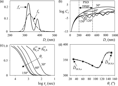
Figure 1. The ill-conditioned problem. (a) Two arbitrary PSDs. (b) Mie coefficients corresponding to nanometric particles (at 5 angles). (c) Normalized autocorrelation measurements. (d) Derived DLS average diameters.

Figure 2. PSD estimation from MDLS measurements: schematic data treatment paths.

Figure 2. PSD estimation from MDLS measurements: schematic data treatment paths.

Table 1. Simulated examples.

Figure 3. Simulated example for the PSD f1. (a) Average diameters i) calculated from the ‘noisy’ MDLS measurements (dots), and ii) simulated with the estimated PSDs. (b, c) The simulated PSD and its estimates from the TI method (b) and m-BI method (c). (d) Estimated PSD obtained from the m-BI method and the standard deviations calculated from the samples obtained through the Metropolis–Hasting algorithm.
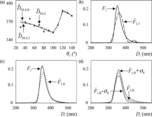
Figure 3. Simulated example for the PSD f1. (a) Average diameters i) calculated from the ‘noisy’ MDLS measurements (dots), and ii) simulated with the estimated PSDs. (b, c) The simulated PSD and its estimates from the TI method (b) and m-BI method (c). (d) Estimated PSD obtained from the m-BI method and the standard deviations calculated from the samples obtained through the Metropolis–Hasting algorithm.
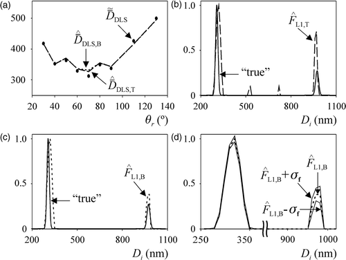
Figure 4. Simulated example for the PSD f2. (Legends as in ).

Figure 4. Simulated example for the PSD f2. (Legends as in Figure 3).

Figure 5. Experimental example for latex L1. (a) Average diameters i) calculated through the cumulants method Citation16 (dots), and ii) simulated with the estimated PSDs. (b, c) Comparison of the ‘true’ PSD with its estimates from the TI method (b) and m-BI method (c). (d) Estimated PSD obtained from the m-BI method and the standard deviations calculated from the samples obtained through the Metropolis–Hasting algorithm.
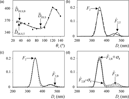
Figure 5. Experimental example for latex L1. (a) Average diameters i) calculated through the cumulants method Citation16 (dots), and ii) simulated with the estimated PSDs. (b, c) Comparison of the ‘true’ PSD with its estimates from the TI method (b) and m-BI method (c). (d) Estimated PSD obtained from the m-BI method and the standard deviations calculated from the samples obtained through the Metropolis–Hasting algorithm.
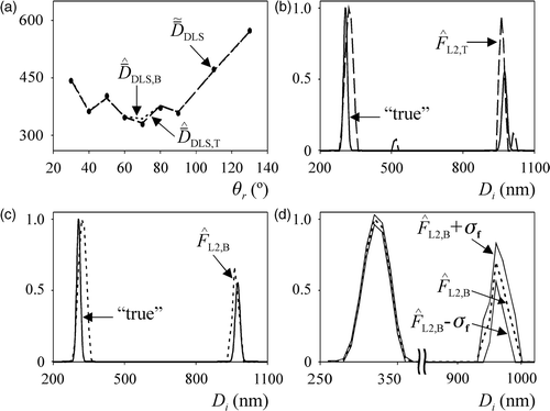
Figure 6. Experimental example for latex L2. (Legends as in ).

Figure 6. Experimental example for latex L2. (Legends as in Figure 5).

Table 2. Experimental examples.

Reprints and Corporate Permissions

Please note: Selecting permissions does not provide access to the full text of the article, please see our help page How do I view content?

To request a reprint or corporate permissions for this article, please click on the relevant link below:

Academic Permissions

Please note: Selecting permissions does not provide access to the full text of the article, please see our help page How do I view content?

Obtain permissions instantly via Rightslink by clicking on the button below:

If you are unable to obtain permissions via Rightslink, please complete and submit this Permissions form. For more information, please visit our Permissions help page.