Figures & data
Figure 1. Inverse results using N = 4 using errorless data: (a) temperature and (b) heat flux inverse predictions.
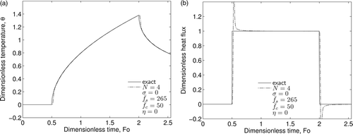
Figure 2. Effect of the sampling rate on the inverse heat flux prediction with N = 7 using errorless data: (a) and (b)
.
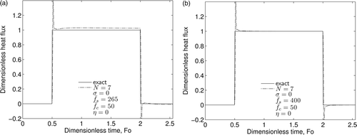
Figure 3. Technique for estimating the noise present in the data: (a) first-order fit to data; (b) least-squares fit to residual; and (c) actual and estimated noises.
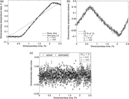
Figure 4. Gaussian low-pass filter exploration: (a) optimum cut-off frequency range and (b) insensitivity of Gaussian filter to a small change in cut-off frequency.
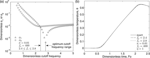
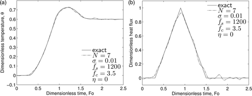
Figure 5. Inverse results using a normal distribution, with a standard deviation of 0.01 and a dimensionless cut-off frequency of 2.6: (a) noisy data used as input to the inverse code; (b) inverse temperature results and (c) inverse heat flux results.
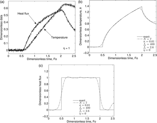
Figure 6. Temperature data for Beck triangle problem: (a) raw data with σ = 0.01 and (b) insensitivity of Gaussian filter to change in cut-off frequency.
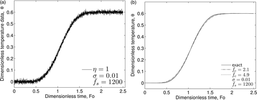
Figure 7. Inverse results for the classical Beck triangle problem for: (a) surface temperature prediction and (b) surface heat flux prediction. Noise was simulated using a normal distribution, σ = 0.01 and used for regularization.