279
Views
3
CrossRef citations to date
0
Altmetric
Original Articles

Practical considerations when using sparse grids with Bayesian inference for parameter estimation

&
Pages 591-608 | Received 28 Feb 2012, Accepted 10 Mar 2012, Published online: 01 May 2012

Figures & data

Figure 1. Comparison of the pdf () for Problem 1.

Figure 1. Comparison of the pdf () for Problem 1.

Figure 2. Effect of ill-conditioning on Bayesian inference for Problem 1.

Figure 2. Effect of ill-conditioning on Bayesian inference for Problem 1.

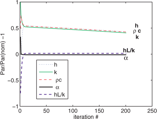
Figure 3. History of iterations using β = 0.01 for Problem 1 when ill-conditioned.

Figure 3. History of iterations using β = 0.01 for Problem 1 when ill-conditioned.

Table 1. Effect of β for σ = 1% (true values: k = 1.0,  h = 1.0, ρc = 20.0 Bi = 1.0, α = 0.05).

Figure 4. Solution trajectories for Problem 1 using exact solutions (solid line) and a sparse grid (dashed line) for two parameters of level 3 (29 sample points) for interpolation.
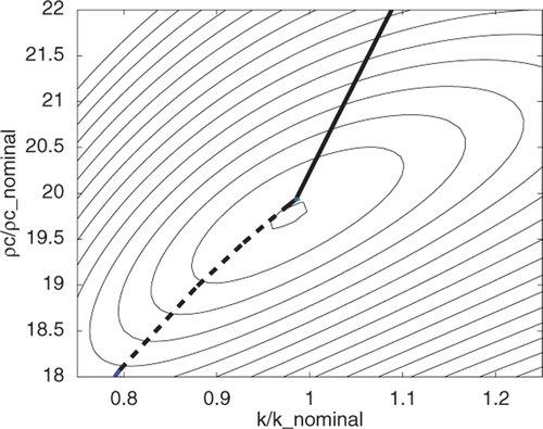
Figure 4. Solution trajectories for Problem 1 using exact solutions (solid line) and a sparse grid (dashed line) for two parameters of level 3 (29 sample points) for interpolation.

Figure 5. Schematic of the panel (thermocouples are placed at the numbered points).

Figure 5. Schematic of the panel (thermocouples are placed at the numbered points).

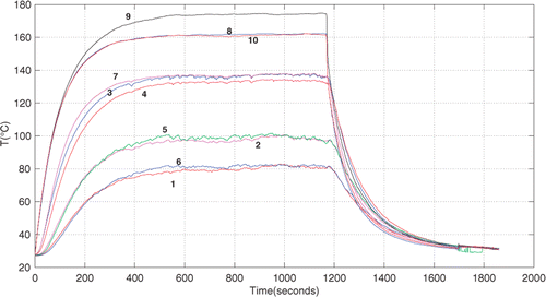
Figure 6. Time history of panel temperatures (numbers denote the thermocouples shown in ).

Figure 6. Time history of panel temperatures (numbers denote the thermocouples shown in Figure 5).

Figure 7. Contours of L(Θ) showing the solution trajectories for Problem 2 using exact solutions of M(Θ) (–-) and interpolation by a sparse grid of level 3 (69 sample points) (- - -).
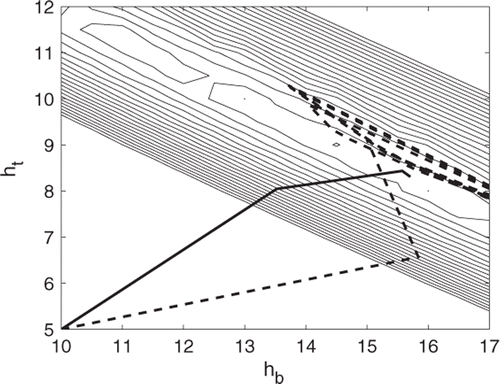
Figure 7. Contours of L(Θ) showing the solution trajectories for Problem 2 using exact solutions of M(Θ) (–-) and interpolation by a sparse grid of level 3 (69 sample points) (- - -).

Figure 8. Level 1 and level 2 sparse grid points: (a) level 1 points (O) and (b) level 2 additional points (X).
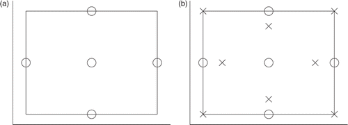
Figure 8. Level 1 and level 2 sparse grid points: (a) level 1 points (O) and (b) level 2 additional points (X).

Figure 9. Reduction in maximum errors of T and ∂T/∂k as a function of sparse grid level for Problem 1 (maximum errors evaluated at x/L = [0, 0.25, 0.5, 0.75, 1.0], Fo = [0 : 1 : 41] (‘spinterp’ results evaluated at x/L = 0.5, Fo = 21).

Figure 9. Reduction in maximum errors of T and ∂T/∂k as a function of sparse grid level for Problem 1 (maximum errors evaluated at x/L = [0, 0.25, 0.5, 0.75, 1.0], Fo = [0 : 1 : 41] (‘spinterp’ results evaluated at x/L = 0.5, Fo = 21).

Figure 10. Interpolated values for sparse grids of increasing levels for Problem 1 using the Chebyshev grid (numbers denote the level): (a) T at x/L = 0.5, Fo = 21 and (b) ∂T/∂k at x/L = 0.5, Fo = 21.
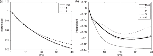
Figure 10. Interpolated values for sparse grids of increasing levels for Problem 1 using the Chebyshev grid (numbers denote the level): (a) T at x/L = 0.5, Fo = 21 and (b) ∂T/∂k at x/L = 0.5, Fo = 21.

Figure 11. Interpolated values for sparse grids of increasing levels for Problem 1 using the Clenshaw–Curtis grid (numbers denote the level): (a) T at x/L = 0.5, Fo = 21 and (b) ∂T/∂k at x/L = 0.5, Fo = 21.
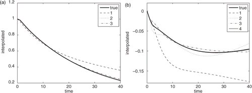
Figure 11. Interpolated values for sparse grids of increasing levels for Problem 1 using the Clenshaw–Curtis grid (numbers denote the level): (a) T at x/L = 0.5, Fo = 21 and (b) ∂T/∂k at x/L = 0.5, Fo = 21.

Figure 12. Interpolation error for the temperature at x/L = 0.5, Fo = 21, Problem 1: (a) Clenshaw–Curtis grid and (b) Chebyshev grid. Interpolation error for the ∂T/∂k at x/L = 0.5, Fo = 21, Problem 1: (c) Clenshaw–Curtis grid and (d) Chebyshev grid.
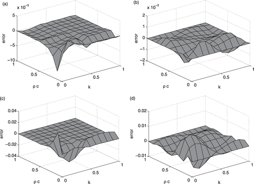
Figure 12. Interpolation error for the temperature at x/L = 0.5, Fo = 21, Problem 1: (a) Clenshaw–Curtis grid and (b) Chebyshev grid. Interpolation error for the ∂T/∂k at x/L = 0.5, Fo = 21, Problem 1: (c) Clenshaw–Curtis grid and (d) Chebyshev grid.

Figure 13. Trajectory for different ways of determining the sensitivities: Exact, solving using the model; SG-a, finite differencing interpolated temperatures; SG-b, differentiating interpolating polynomials representing temperature; SG-c, interpolating sensitivities.
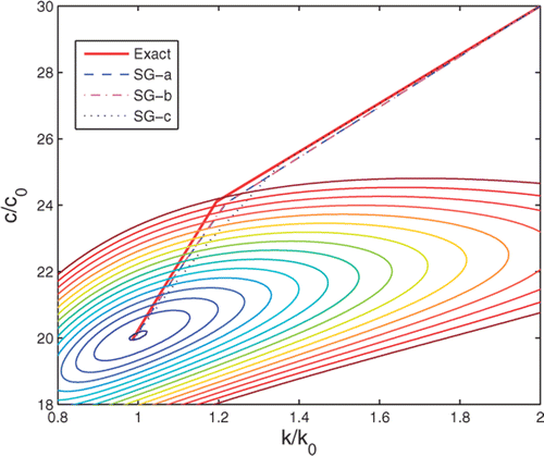
Figure 13. Trajectory for different ways of determining the sensitivities: Exact, solving using the model; SG-a, finite differencing interpolated temperatures; SG-b, differentiating interpolating polynomials representing temperature; SG-c, interpolating sensitivities.

Figure 14. Effect of refining the range of parameters for in Problem 1 (ρc specified): (a) expanded range and (b) centred about LS solution using sparse grid interpolation.
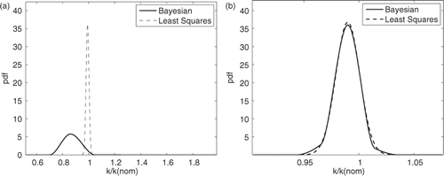
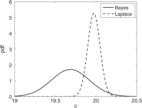
Figure 14. Effect of refining the range of parameters for in Problem 1 (ρc specified): (a) expanded range and (b) centred about LS solution using sparse grid interpolation.
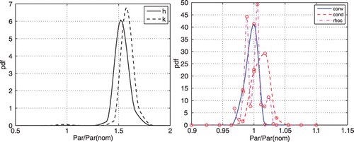
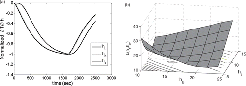
Figure 15. Behaviour of the panel: (a) time history of sensitivity of temperature and (b) surface of L(ht, hb) for the panel at TC 9.

Figure 15. Behaviour of the panel: (a) time history of sensitivity of temperature and (b) surface of L(ht, hb) for the panel at TC 9.

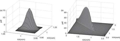
Figure 16. Joint probability densities for Problem 1: (a) well-conditioned and (b) ill-conditioned.

Figure 16. Joint probability densities for Problem 1: (a) well-conditioned and (b) ill-conditioned.

Reprints and Corporate Permissions

Please note: Selecting permissions does not provide access to the full text of the article, please see our help page How do I view content?

To request a reprint or corporate permissions for this article, please click on the relevant link below:

Academic Permissions

Please note: Selecting permissions does not provide access to the full text of the article, please see our help page How do I view content?

Obtain permissions instantly via Rightslink by clicking on the button below:

If you are unable to obtain permissions via Rightslink, please complete and submit this Permissions form. For more information, please visit our Permissions help page.