Reduced forward models in electrical impedance tomography with probe geometry

Figures & data

Figure 1. A schematic picture of the measurement probe and the computation domain. The ring-shaped electrodes (black rings) are shown on the boundary of the probe. The radius of the probe $r_0=3$ cm, radius of the computation domain $R=25$ cm and height of the domain $z_2-z_1=94$ cm. The four points indicated in the figure define the rz-plane in which the 2D reconstructions are computed. Furthermore, the cross-sections of the 3D reconstructions that are shown in Section 4 are represented on the same rz-plane.

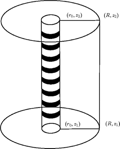
Figure 2. (a) The computation domain and the measurement probe. The electrodes are shown with black patches. In some inverse solutions, the conductivity is assumed to be homogeneous in the upper and bottom parts of the computation domain. The cutting planes of the homogeneous parts are shown with dashed horizontal lines (location in the $z$-axis is $z=20$ and $z=74$). (b) A prior covariance matrix for 1D reconstructions (correlation length ${\mathit{\beta }}_{\mathrm{z}}=5$ cm and variance $a=1000$). (c) A prior covariance matrix for 1D reconstructions (correlation length ${\mathit{\beta }}_{\mathrm{z}}=15$ cm and variance $a=1000$).

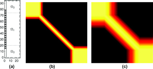
Figure 3. Simulated conductivities used for the simulation of the measurements.

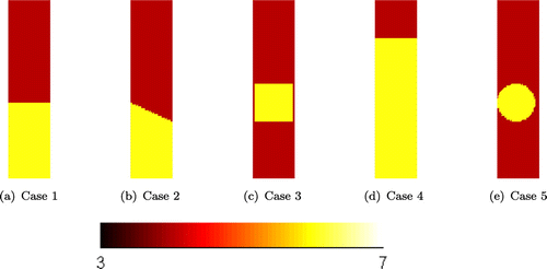
Table 1. Finite element meshes, where $N_n$ is the number of nodes, $N_e$ the number of elements in meshes and basis is the basis functions used for the conductivity.

Mesh	$N_n$	$N_e$	Basis	Usage
${\mathcal{M}}_{\mathrm{s}im}$	72,484	365,977	Linear	Simulation of measurements
${\mathcal{M}}_{3D}$	33,225	167,928	Linear	3D model
${\mathcal{M}}_{3D,\mathrm{i}nv}$	3448	16,170	Linear	3D inversion
${\mathcal{M}}_{2D}$	2280	4324	Constant	2D model
${\mathcal{M}}_{1D}$	941	940	Constant	1D model

Figure 4. The simulated voltages for the Case 1. (a) All simulated voltages corresponding to current injection between the first and last electrodes are shown. (b) Only the voltages measured near the interface in the conductivity are shown. The voltages shown with blue (thick line), red (thin line) and black (dashed line) are computed with 3D, 2D and 1D models, respectively.

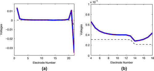
Figure 5. (a) The average percentual modelling error level between 3D and 1D model. (b) The average percentual modelling error level between 3D and 2D cylindrically symmetric model. The mean is shown with blue line and standard deviation with thick red line.

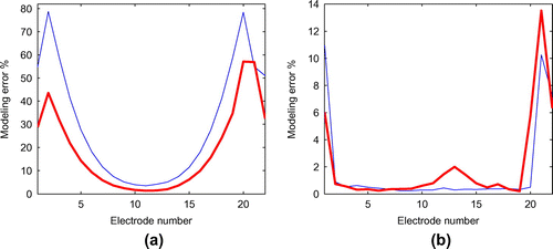
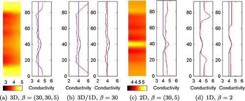
Figure 6. The cross-sections of the 3D reconstructions (Case 1) and vertical conductivity profiles (mean of the 3D conductivity (2121 $$\begin{array}{c}\hfill \mathit{\sigma }(z)=\frac{1}{R-r_0}{\int }_{r_0}^R\mathit{\sigma }(r,z)dr={\tilde{P}}_{1D}{P}_{2D}\overline{\mathit{\sigma }}=P_{1D}\overline{\mathit{\sigma }},\end{array}$$21 )). $\mathit{\beta }$ refers to the correlation length ($\mathit{\beta }=({\mathit{\beta }}_x,{\mathit{\beta }}_y,{\mathit{\beta }}_z)$) in the prior model (2929 $$\begin{array}{c}\hfill {\mathrm{\Gamma }}_{\mathrm{p}}r(i,j)=\left\{\begin{array}{cc}\hfill aexp\left\{-,\sum _{k=1}^{\mathrm{d}im},\frac{{\left(x_k^i,-,x_k^j\right)}^2}{2{\mathit{\beta }}_k^2}\right\}+{\mathit{\mu }}_{\mathrm{hg}}^2& ,\forall x_k^i,x_k^j\in {\mathrm{\Omega }}_1,\hfill \\ \hfill {\mathit{\mu }}_{\mathrm{hg}}^2& ,\forall x_k^i,x_k^j\in {\mathrm{\Omega }}_2,\hfill \\ \hfill aexp\left\{-,\sum _{k=1}^{\mathrm{d}im},\frac{{\left(x_k^i,-,x_k^l\right)}^2}{2{\mathit{\beta }}_k^2}\right\}+{\mathit{\mu }}_{\mathrm{hg}}^2& ,\forall x_k^i\in {\mathrm{\Omega }}_1,x_k^j\in {\mathrm{\Omega }}_2.\hfill \end{array}\right.\end{array}$$29 ) and ${\mathrm{\Delta }}_{\mathit{\sigma }}$ (%) are the relative reconstruction errors (3333 $$\begin{array}{c}\hfill {\mathrm{\Delta }}_{\mathit{\sigma }}=\frac{\mid \mid P_{1}D{\mathit{\sigma }}_{\mathrm{t}}rue-P_i{\mathit{\sigma }}_{\mathrm{M}AP}\mid \mid }{\mid \mid P_{1}D{\mathit{\sigma }}_{\mathrm{t}}rue\mid \mid }\times 100\%,\end{array}$$33 ).

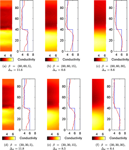
Table 2. Average computation times (s) for inverse problem using 1D, 2D, 3D-models and 3D/1D approach in Case 1.

	1D	2D	3D	3D/1D
Computation time	7	180	400	356

Figure 7. The estimated vertical conductivity profiles (Case 1) (3D/1D reconstructions). $\mathit{\beta }$ refers to correlation length ($\mathit{\beta }={\mathit{\beta }}_z$) in the prior model. On the right hand side estimates the conductivity is modelled to be homogeneous at the top and bottom end of the computation domain. ${\mathrm{\Delta }}_{\mathit{\sigma }}$ (%) are the relative reconstruction errors (3333 $$\begin{array}{c}\hfill {\mathrm{\Delta }}_{\mathit{\sigma }}=\frac{\mid \mid P_{1}D{\mathit{\sigma }}_{\mathrm{t}}rue-P_i{\mathit{\sigma }}_{\mathrm{M}AP}\mid \mid }{\mid \mid P_{1}D{\mathit{\sigma }}_{\mathrm{t}}rue\mid \mid }\times 100\%,\end{array}$$33 ). The first relative reconstruction errors are for the left figures and the second ones are for the right figures.

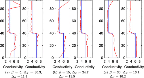
Figure 8. The 2D reconstructions (Case 1) and vertical conductivity profiles (mean of the 2D conductivity). $\mathit{\beta }$ refers to correlation length ($\mathit{\beta }=({\mathit{\beta }}_r,{\mathit{\beta }}_z)$) in the prior model and ${\mathrm{\Delta }}_{\mathit{\sigma }}$ (%) are the relative reconstruction errors (3333 $$\begin{array}{c}\hfill {\mathrm{\Delta }}_{\mathit{\sigma }}=\frac{\mid \mid P_{1}D{\mathit{\sigma }}_{\mathrm{t}}rue-P_i{\mathit{\sigma }}_{\mathrm{M}AP}\mid \mid }{\mid \mid P_{1}D{\mathit{\sigma }}_{\mathrm{t}}rue\mid \mid }\times 100\%,\end{array}$$33 ).

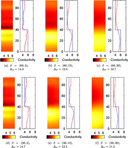
Figure 9. The 1D reconstructions (Case 1) with the approximation error approach are shown on the top row and 1D MAP-CEM reconstructions (without approximation error approach) on the bottom row. $\mathit{\beta }$ refers to the correlation length ($\mathit{\beta }={\mathit{\beta }}_z$) in the prior model. On the right hand side estimates the conductivity is modelled to be homogeneous at the ends of the computation domain. ${\mathrm{\Delta }}_{\mathit{\sigma }}$ (%) are the relative reconstruction errors (3333 $$\begin{array}{c}\hfill {\mathrm{\Delta }}_{\mathit{\sigma }}=\frac{\mid \mid P_{1}D{\mathit{\sigma }}_{\mathrm{t}}rue-P_i{\mathit{\sigma }}_{\mathrm{M}AP}\mid \mid }{\mid \mid P_{1}D{\mathit{\sigma }}_{\mathrm{t}}rue\mid \mid }\times 100\%,\end{array}$$33 ). The first relative reconstruction errors are for the left figures and the second ones are for the right figures.

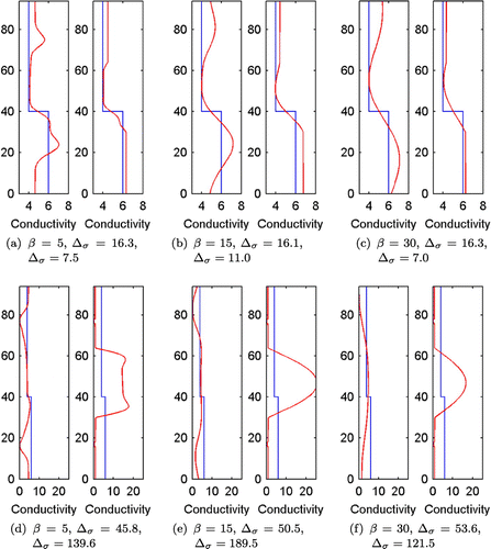
Figure 10. The estimated conductivities (Case 2). (a) 3D reconstructions (b) 3D/1D reconstruction (c) 2D reconstruction (d) 1D reconstruction.

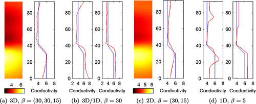
Figure 11. The sensitivity of the measurements in logarithmic scale (sum of absolute values of all rows in Jacobian matrix) with two different current patterns. (a) The adjacent current and measurement patterns that were used in the simulations. (b) The opposite current pattern and adjacent measurement pattern were used. The opposite current pattern was used in one test case, see Figure 12.

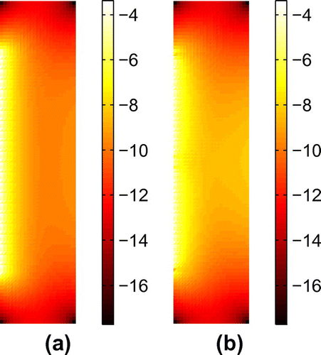
Figure 12. Estimated conductivity using 2D model with opposite current patterns. The correlation length was $\mathit{\beta }=(30,15)$.

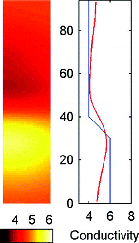
Figure 13. Estimated conductivities (Case 3). (a) 3D reconstruction (b) 3D/1D reconstruction (c) 2D reconstruction (d) 1D reconstruction.

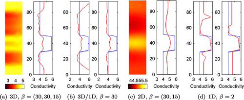
Figure 14. Estimated conductivities (Case 4). (a) 3D reconstruction (b) 3D/1D reconstruction (c) 2D reconstruction (d) 1D reconstruction (length of the homogeneous regions is 30 cm).

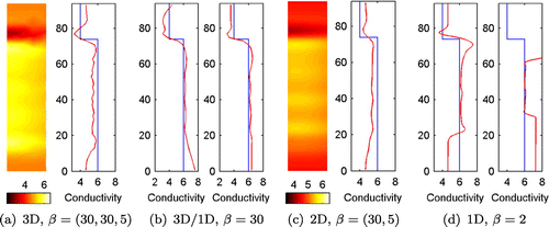
Figure 15. 1D reconstruction (Case 4), correlation length $\mathit{\beta }=2$. Length of the homogeneous regions is 15 cm.

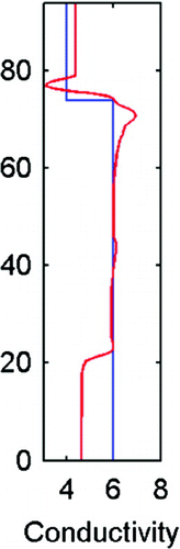
Figure 16. The estimated conductivities (Case 5). (a) 3D reconstruction (b) 3D/1D reconstruction (c) 2D reconstruction (d) 1D reconstruction.