Elasticity imaging of biological soft tissue using a combined finite element and non-linear optimization method

Figures & data

Figure 1. (a) The geometry and boundary conditions of the FE model, (b) FE mesh.

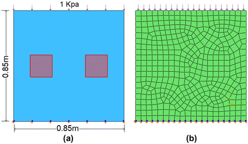
Figure 2. (a) The geometry and boundary conditions of the FE model, (b) FE mesh.

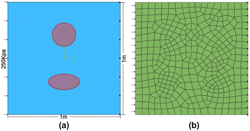
Figure 3. Contours of the normal strain in the vertical direction.

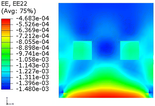
Figure 4. (a1)(a2) Estimated and final parameters obtained with exact displacement data, (b1)(b2) Estimated and final parameters obtained with ±1% noise added, (c1)(c2) Estimated and final parameters obtained with ±3% noise added.

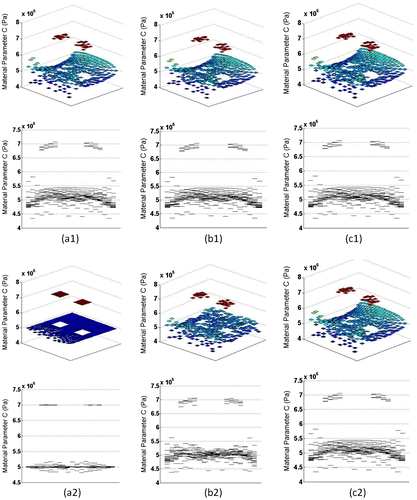
Table 1. Sensitivity study result when different level of noise is added.

Condition	Initial guess				Final convergence
	Objective cost (R)	Relative error in stiffness (%)			Objective cost (R)	Relative error in stiffness (%)
		Min	Mean	Max		Min	Mean	Max
Exact data with no noise	5.07e − 6	7.21e − 3	3.26	16.42	1.37e − 11	2.43e − 5	0.29	3.60
Exact data with ±1% noise	8.52e − 6	7.21e − 3	3.26	16.42	3.40e − 6	0.01	2.32	12.56
Exact data with ±3% noise	3.49e − 5	7.21e − 3	3.26	16.42	3.49e − 5	7.21e − 3	3.26	16.42

Figure 5. Contour of the normal strain in the horizontal direction.

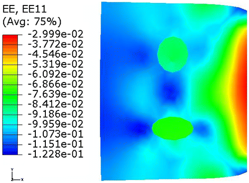
Figure 6. (a1)(b1) Estimated and final parameters obtained with exact displacement data, (a2)(b2) Estimated and final parameters obtained with ±0.5% noise added.

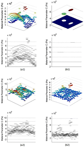
Table 2. Sensitivity study result when different level of noise is added.

Condition	Initial guess				Final convergence
	Objective cost (R)	Relative error in stiffness (%)			Objective cost (R)	Relative error in stiffness (%)
		Min	Mean	Max		Min	Mean	Max
Exact data with no noise	1.74e − 2	4.76e − 2	26.35	108.13	5.29e − 13	6.78e − 6	2.95e − 3	2.03e − 2
Exact data with ±0.5% noise	2.92e − 2	0.91	31.57	144.91	0.56e − 5	0.14e − 2	9.19	48.66

Table 3. Computational time. Method 1: proposed method. Method 2: pure optimization method (uniform initial guess, finite difference to calculated Jacobian matrix).

Methods	Model in Section 3.2		Model in Section 3.3
	Iteration number	Execution time	Iteration number	Execution time
Method 1	8	5 min	6	3 min
Method 2	16	>6 h	10	>6 h

Figure 7. Images of human lower leg (a) MR image, white circle represents the indenter, blue arrow represents the indentation direction, (b) FE boundary conditions.

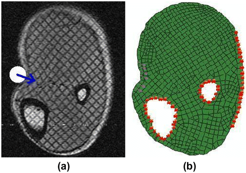
Figure 8. (a) Measured displacement in the horizontal direction, (b) Measured displacement in the vertical direction.

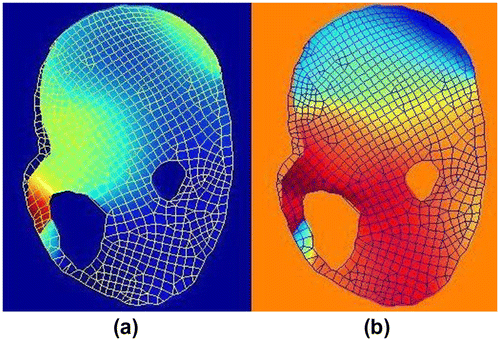
Figure 9. Elastography of human lower leg (Material Parameter: C, unit: kPa).

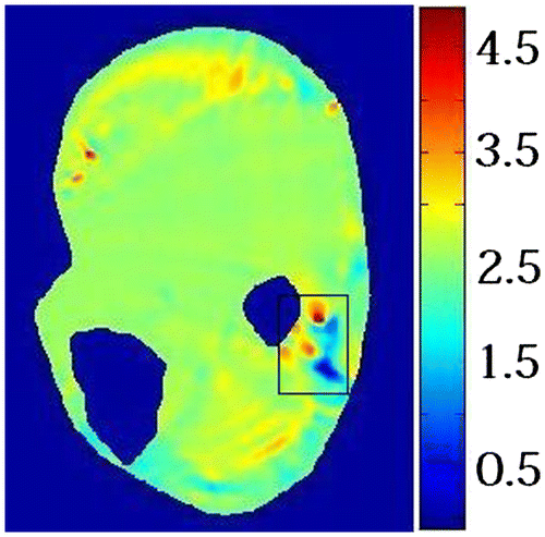
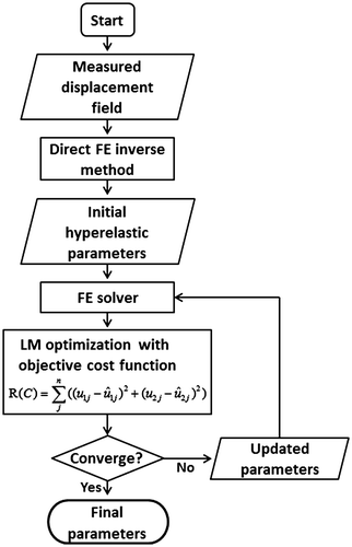
Figure 10. Flowchart of the combined finite element and non-linear optimization method.