Comparative numerical analysis of identification problems related to nonlinear transport-diffusion model of a settler

Figures & data

Figure 1. A schematic outline of an wastewater treatment plant.

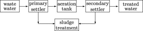
Figure 2. The behaviour of the density function $u(x,t)$ for Model A given in test Example 1.

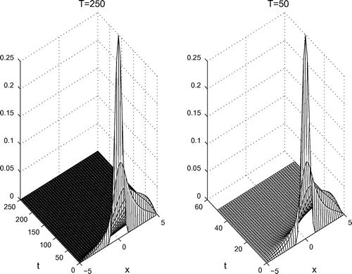
Figure 3. Exact solution $c(x)$ and numerical approximation $c^{(n)}(x)$ and the behaviour of the errors $e(n)$ for test Example 1.

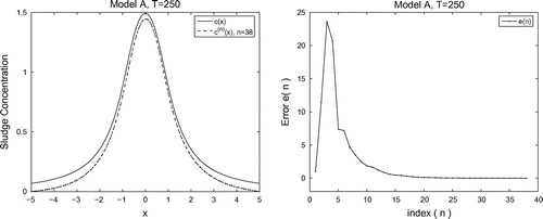
Figure 4. An influence of variable diffusion coefficients $D(x)$ to the sludge concentration $c(x)$.

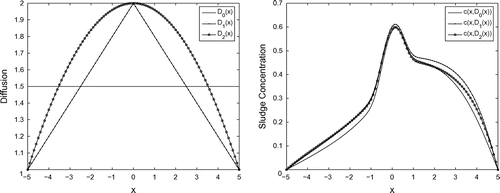
Table 1. Results of computational experiments for the Model A.

Final time ($T$)	$N$	$M$	$h_x$	$h_t$	$\frac{\Vert u-u_h{\Vert }_{\infty }}{{\Vert u\Vert }_{\infty }}$	$\frac{\Vert c-c_h{\Vert }_{\infty }}{{\Vert c\Vert }_{\infty }}$	Number of iterations
50	21	26	0.5	2.0	$6.29\times {10}^{-2}$	$1.38\times {10}^{-1}$	24
250	21	84	0.5	3.0	$\mathbf{5}.\mathbf{53}\times {\mathbf{10}}^{-\mathbf{2}}$	$\mathbf{8}.\mathbf{04}\times {\mathbf{10}}^{-\mathbf{2}}$	25
250	21	251	0.5	1.0	$5.57\times {10}^{-2}$	$8.24\times {10}^{-2}$	34
500	21	101	0.5	5.0	$7.74\times {10}^{-2}$	$2.1\times {10}^{-1}$	20
500	21	501	0.5	1.0	$\mathbf{5}.\mathbf{26}\times {\mathbf{10}}^{-\mathbf{2}}$	$\mathbf{6}.\mathbf{88}\times {\mathbf{10}}^{-\mathbf{2}}$	35
500	41	501	0.25	1.0	$2.27\times {10}^{-2}$	$4.65\times {10}^{-2}$	38

Figure 5. An influence of the settling velocity $\mathit{\nu }(t)$ to the sludge concentration $c(x)$.

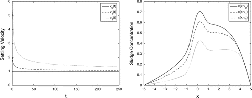
Table 2. Results of computational experiments for the Model B.

Final time ($T$)	$N$	$M$	$h_x$	$h_t$	$\frac{\Vert u-u_h{\Vert }_{\infty }}{{\Vert u\Vert }_{\infty }}$	$\frac{\Vert c-c_h{\Vert }_{\infty }}{{\Vert c\Vert }_{\infty }}$	Number of iterations
50	21	26	0.5	2.0	$\mathbf{4}.\mathbf{40}\times {\mathbf{10}}^{-\mathbf{2}}$	$\mathbf{1}.\mathbf{78}\times {\mathbf{10}}^{-\mathbf{1}}$	5
50	41	51	0.25	1.0	$1.92\times {10}^{-2}$	$1.90\times {10}^{-1}$	6
250	21	251	0.5	1.0	$2.86\times {10}^{-2}$	$8.58\times {10}^{-2}$	6
250	41	251	0.25	1.0	$\mathbf{1}.\mathbf{90}\times {\mathbf{10}}^{-\mathbf{2}}$	$\mathbf{8}.\mathbf{53}\times {\mathbf{10}}^{-\mathbf{2}}$	6
500	21	101	0.5	5.0	$5.41\times {10}^{-2}$	$2.74\times {10}^{-1}$	5
500	21	501	0.5	1.0	$\mathbf{2}.\mathbf{88}\times {\mathbf{10}}^{-\mathbf{2}}$	$\mathbf{6}.\mathbf{44}\times {\mathbf{10}}^{-\mathbf{2}}$	6

Figure 6. The ‘square wave’ initial density function $u(x,0)=\mathit{\phi }(x)$ (the left figure) and the corresponding solution $c^{(n)}(x)$ (the right figure) of the identification problem (17) in the Model B.

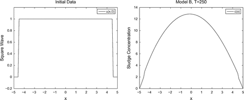
Figure 7. The behaviour of the density function $u(x,t)$ for Model B.

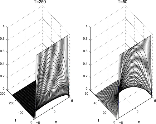
Figure 8. Behavior of the sludge concentration $c(x)$ for various values of the maximum settling velocity ${\mathit{\nu }}_0>0$ and the model parameter ${\mathit{\alpha }}_0>0$, given in [17], and for different initial data.

Figure 9. Comparative analysis of the models: The behaviour of the sludge concentration function $c(x)$.

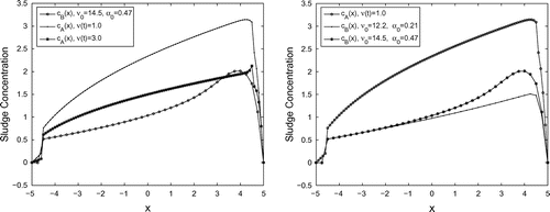
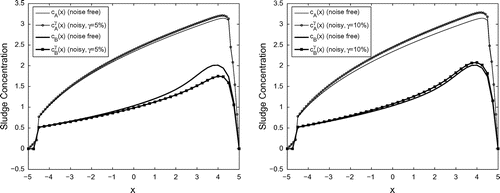
Figure 10. Comparative analysis of the models: Noise free($c_A,c_B$) and noisy ($c_A^{\mathit{\gamma }},c_B^{\mathit{\gamma }}$).

Smolianski A, Shipilova O, Haario H. A fast high-resolution algorithm for linear convection problems: particle transport method. Int. J. Numer. Meth. Eng. 2007;70:655–684.

 Web of Science ®Google Scholar