253
Views
2
CrossRef citations to date
0
Altmetric
Articles

A Slepian framework for the inverse problem of equivalent gravitational potential generated by discrete point masses

, &
Pages 331-350 | Received 19 Jun 2012, Accepted 01 Dec 2013, Published online: 24 Apr 2014

Figures & data

Figure 1. A schematic of the positions of the two point-masses.

Figure 1. A schematic of the positions of the two point-masses.

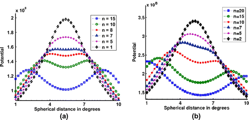
Figure 2. Plots of the potential on the observation sphere (R~=Rm+30km,Rm=6378km) as function of the distance between the point masses. The coordinates are given by ψi=ψ0±niΔψ where Δψ=0.2308.

Figure 2. Plots of the potential on the observation sphere (R~=Rm+30km,Rm=6378km) as function of the distance between the point masses. The coordinates are given by ψi=ψ0±niΔψ where Δψ=0.2308∘.

Figure 3. Gaussian curvature of the potential as function of the spherical distance between the point masses. (a) corresponds to the case of equal masses. (b) represents the case of two different masses.
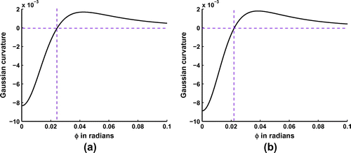
Figure 3. Gaussian curvature of the potential as function of the spherical distance between the point masses. (a) corresponds to the case of equal masses. (b) represents the case of two different masses.

Figure 4. A schematic of both cases studied in Section 4.2. In (a), we show the principal retrieved point-mass (P0,m0) and the masses identified when adding noise. In (b), we show the second experiment dealing with identifying two point masses (P1,m1)and(P2,m2), and we see the masses identified around the principal masses. The difference between the found point masses sizes is shown in both cases.
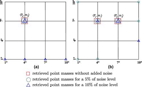
Figure 4. A schematic of both cases studied in Section 4.2. In (a), we show the principal retrieved point-mass (P0,m0) and the masses identified when adding noise. In (b), we show the second experiment dealing with identifying two point masses (P1,m1)and(P2,m2), and we see the masses identified around the principal masses. The difference between the found point masses sizes is shown in both cases.

Table 1. Influence of the level of the added noise on the retrieved mass values. In the second and the third columns we give the ratios of the retrieved principal masses and the initial masses.

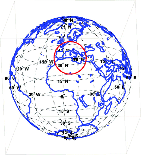
Figure 5. The geographic region under study (circle) which is a spherical cap centred at the point with longitude 10W and latitude 34N.

Figure 5. The geographic region under study (circle) which is a spherical cap centred at the point with longitude 10∘W and latitude 34∘N.

Figure 6. Slepian functions for the spherical cap with Θ45 and with bandlimit L=30. The first two rows show the Slepian functions corresponding to the first six largest eigenvalues. The last row shows those Slepian functions which correspond to very small eigenvalues.
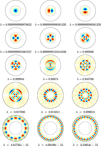
Figure 6. Slepian functions for the spherical cap with Θ≤45∘ and with bandlimit L=30. The first two rows show the Slepian functions corresponding to the first six largest eigenvalues. The last row shows those Slepian functions which correspond to very small eigenvalues.

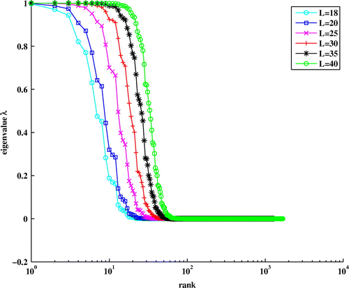
Figure 7. Spectrum of the spatio-spectral concentration problem on the spherical cap with Θ45 (domain under study) and bandwidth L=18,20,25,30,35,40. On the x-axis, we show the rank of the eigenvalues and on the y-axis their magnitudes.

Figure 7. Spectrum of the spatio-spectral concentration problem on the spherical cap with Θ≤45∘ (domain under study) and bandwidth L=18,20,25,30,35,40. On the x-axis, we show the rank of the eigenvalues and on the y-axis their magnitudes.

Figure 8. The grid that we use in the computations consists of a web of points regularly spaced in both the radial and tangential directions. The minimal distances between the points of this grid respect the stability condition.
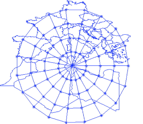
Figure 8. The grid that we use in the computations consists of a web of points regularly spaced in both the radial and tangential directions. The minimal distances between the points of this grid respect the stability condition.
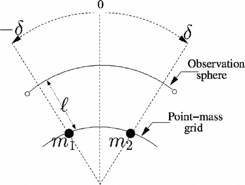
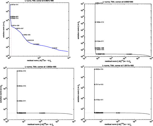
Figure 9. L-curves for the initial guess, and at iteration numbers 2, 6 and 12. The value of the optimal regularisation parameter is given by the value of this parameter at the corner of the L-shape.

Figure 9. L-curves for the initial guess, and at iteration numbers 2, 6 and 12. The value of the optimal regularisation parameter is given by the value of this parameter at the corner of the L-shape.

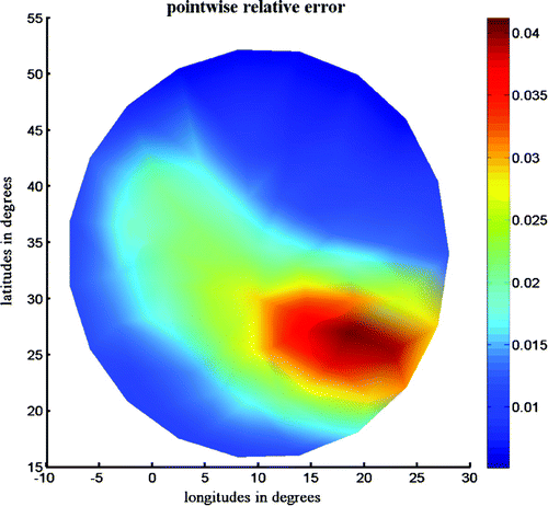
Figure 10. Results of pointwise relative error between the given and the approximated gravitational potentials on the studied grid.

Figure 10. Results of pointwise relative error between the given and the approximated gravitational potentials on the studied grid.

Reprints and Corporate Permissions

Please note: Selecting permissions does not provide access to the full text of the article, please see our help page How do I view content?

To request a reprint or corporate permissions for this article, please click on the relevant link below:

Academic Permissions

Please note: Selecting permissions does not provide access to the full text of the article, please see our help page How do I view content?

Obtain permissions instantly via Rightslink by clicking on the button below:

If you are unable to obtain permissions via Rightslink, please complete and submit this Permissions form. For more information, please visit our Permissions help page.