234
Views
2
CrossRef citations to date
0
Altmetric
Articles

A wavelet multiscale-adaptive homotopy method for the inverse problem of nonlinear diffusion equation

&
Pages 617-634 | Received 16 Apr 2013, Accepted 08 May 2014, Published online: 06 Jun 2014

Figures & data

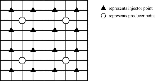
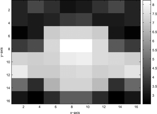
Figure 1. Simulation geometry with the locations of producer points and injector points.

Figure 1. Simulation geometry with the locations of producer points and injector points.

Figure 2. The errors of numerical solution and ground truth with respect to the iteration numbers with different initial values in Example 5.1: (a) the initial value is 0.17; (b) the initial value is 2.45; (c) the initial value is 4.15; (d) the initial value is 6.58.
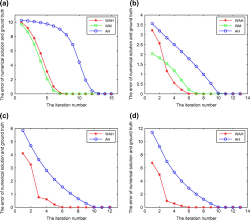
Figure 2. The errors of numerical solution and ground truth with respect to the iteration numbers with different initial values in Example 5.1: (a) the initial value is 0.17; (b) the initial value is 2.45; (c) the initial value is 4.15; (d) the initial value is 6.58.

Figure 3. The numerical solutions with respect to the iteration numbers with the initial value 0.17 at some grid points in Example 5.1: (a) the grid point is (1/8, 1/8); (b) the grid point is (1/8, 7/8); (c) the grid point is (7/8, 1/8); (d) the grid point is (7/8, 7/8).
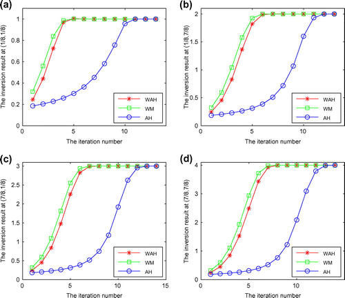
Figure 3. The numerical solutions with respect to the iteration numbers with the initial value 0.17 at some grid points in Example 5.1: (a) the grid point is (1/8, 1/8); (b) the grid point is (1/8, 7/8); (c) the grid point is (7/8, 1/8); (d) the grid point is (7/8, 7/8).
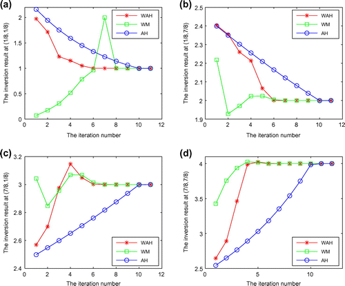
Figure 4. The numerical solutions with respect to the iteration numbers with the initial value 2.45 at some grid points in Example 5.1: (a) the grid point is (1/8, 1/8); (b) the grid point is (1/8, 7/8); (c) the grid point is (7/8, 1/8); (d) the grid point is (7/8, 7/8).

Figure 4. The numerical solutions with respect to the iteration numbers with the initial value 2.45 at some grid points in Example 5.1: (a) the grid point is (1/8, 1/8); (b) the grid point is (1/8, 7/8); (c) the grid point is (7/8, 1/8); (d) the grid point is (7/8, 7/8).

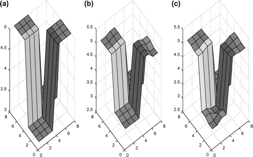
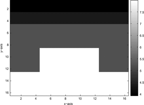
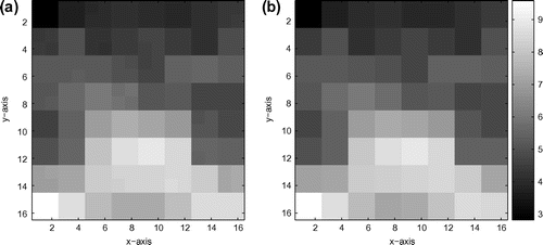
Figure 5. The true model based on (Equation2.2) and inversion results q with the noise level ϵ=0.05 in Example 5.2: (a) the true model based on (Equation2.2); (b) the inversion result q for N(u)=1+0.1|u|2; (c) the inversion result q for N(u)=1/(1-0.1|u|2).

Figure 5. The true model based on (Equation2.22.2 ut-∇·(q(x)N(∇u)∇u)=s(x,t),(x,t)∈Ω×(0,T),2.2 ) and inversion results q∗ with the noise level ϵ=0.05 in Example 5.2: (a) the true model based on (Equation2.22.2 ut-∇·(q(x)N(∇u)∇u)=s(x,t),(x,t)∈Ω×(0,T),2.2 ); (b) the inversion result q∗ for N(∇u)=1+0.1|∇u|2; (c) the inversion result q∗ for N(∇u)=1/(1-0.1|∇u|2).

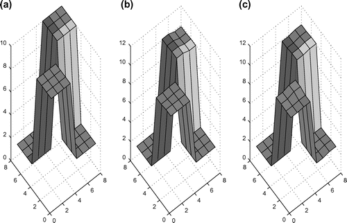
Figure 6. The true model based on (Equation2.1) and inversion results q with the noise level ϵ=0.05 in Example 5.3: (a) the true model based on (Equation2.1); (b) the inversion result q for N(u)=u4-u3+u2-u+1; (c) the inversion result q for N(u)=u4+u3+u2+u+1.

Figure 6. The true model based on (Equation2.12.1 ut-∇·(q(x)N(u)∇u)=s(x,t),(x,t)∈Ω×(0,T),2.1 ) and inversion results q∗ with the noise level ϵ=0.05 in Example 5.3: (a) the true model based on (Equation2.12.1 ut-∇·(q(x)N(u)∇u)=s(x,t),(x,t)∈Ω×(0,T),2.1 ); (b) the inversion result q∗ for N(u)=u4-u3+u2-u+1; (c) the inversion result q∗ for N(u)=u4+u3+u2+u+1.

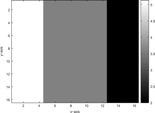
Figure 7. The true model based on (Equation2.1) in Example 5.4.

Figure 7. The true model based on (Equation2.12.1 ut-∇·(q(x)N(u)∇u)=s(x,t),(x,t)∈Ω×(0,T),2.1 ) in Example 5.4.

Figure 8. The inversion result q at the original scale with the noise level ϵ=0.01 in Example 5.4.

Figure 8. The inversion result q∗ at the original scale with the noise level ϵ=0.01 in Example 5.4.

Figure 9. The true model based on (Equation2.2) in Example 5.5.

Figure 9. The true model based on (Equation2.22.2 ut-∇·(q(x)N(∇u)∇u)=s(x,t),(x,t)∈Ω×(0,T),2.2 ) in Example 5.5.

Figure 10. The inversion result q at the original scale with the noise level ϵ=0.01 in Example 5.5.

Figure 10. The inversion result q∗ at the original scale with the noise level ϵ=0.01 in Example 5.5.

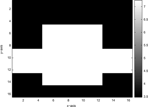
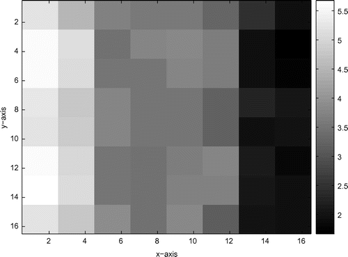
Figure 11. The true model based on (Equation2.1) in Example 5.6.

Figure 11. The true model based on (Equation2.12.1 ut-∇·(q(x)N(u)∇u)=s(x,t),(x,t)∈Ω×(0,T),2.1 ) in Example 5.6.

Figure 12. The inversion results q with the noise level ϵ=0.04 in Example 5.6: (a) the inversion result q at scale 1; (b) the inversion result q at scale 0.

Figure 12. The inversion results q∗ with the noise level ϵ=0.04 in Example 5.6: (a) the inversion result q∗ at scale 1; (b) the inversion result q∗ at scale 0.

Table 1. The errors of numerical solution and ground truth by WAH, WM and AH with the initial value 0.17 in Example 5.1.

Table 2. The errors of numerical solution and ground truth by WAH, WM and AH with the initial value 2.45 in Example 5.1.

Table 3. The errors of numerical solution and ground truth by WAH, WM and AH with the initial value 4.15 in Example 5.1.

Table 4. The errors of numerical solution and ground truth by WAH, WM and AH with the initial value 6.58 in Example 5.1.

Table 5. The required iteration numbers by WAH, WM and AH in Example 5.1.

Table 6. The required CPU times (in seconds) by WAH, WM and AH in Example 5.1.

Reprints and Corporate Permissions

Please note: Selecting permissions does not provide access to the full text of the article, please see our help page How do I view content?

To request a reprint or corporate permissions for this article, please click on the relevant link below:

Academic Permissions

Please note: Selecting permissions does not provide access to the full text of the article, please see our help page How do I view content?

Obtain permissions instantly via Rightslink by clicking on the button below:

If you are unable to obtain permissions via Rightslink, please complete and submit this Permissions form. For more information, please visit our Permissions help page.