1,672
Views
55
CrossRef citations to date
0
Altmetric
Articles

Generalized finite difference method for solving two-dimensional inverse Cauchy problems

, &
Pages 737-759 | Received 25 Sep 2013, Accepted 09 Jun 2014, Published online: 10 Jul 2014

Figures & data

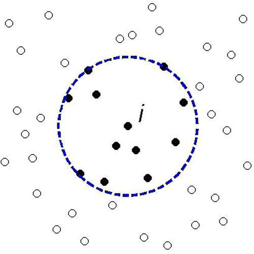
Figure 1. Schematic diagram for the circular shape of the star.

Figure 1. Schematic diagram for the circular shape of the star.

Figure 2. (a) The schematic diagram for example 1 and (b) the distributions of interior and boundary nodes.
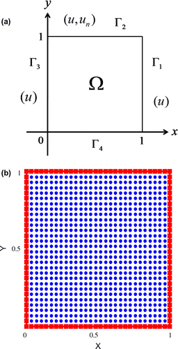
Figure 2. (a) The schematic diagram for example 1 and (b) the distributions of interior and boundary nodes.

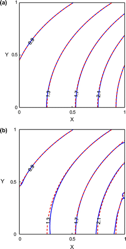
Figure 3. The distributions of numerical (solid lines) and analytical solutions (dashed lines). (a) s=0 and (b) s=3.

Figure 3. The distributions of numerical (solid lines) and analytical solutions (dashed lines). (a) s=0 and (b) s=3.

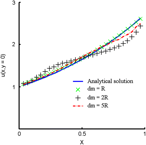
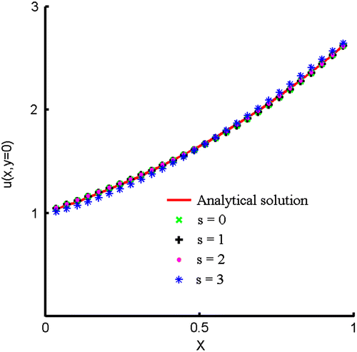
Figure 4. The profiles of numerical solutions along Γ4 for example 1.

Figure 4. The profiles of numerical solutions along Γ4 for example 1.

Table 1. The maximum absolute errors by adding different levels of noise for example 1.

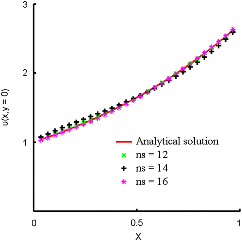
Figure 5. The profiles of numerical solutions along Γ4 for example 1 (s = 3).

Figure 5. The profiles of numerical solutions along Γ4 for example 1 (s = 3).

Figure 6. The profiles of numerical solutions along Γ4 by adopting different supporting radii of weighting function for example 1 (s = 3, ns=12).

Figure 6. The profiles of numerical solutions along Γ4 by adopting different supporting radii of weighting function for example 1 (s = 3, ns=12).

Figure 7. (a) The schematic diagram for example 2 and (b) the distributions of interior and boundary nodes.
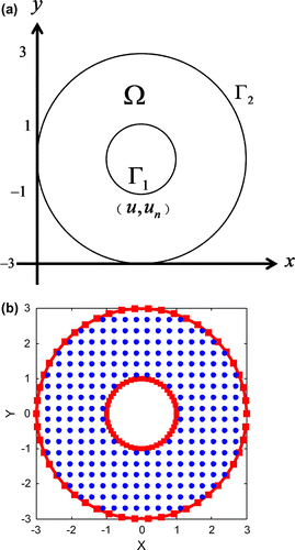
Figure 7. (a) The schematic diagram for example 2 and (b) the distributions of interior and boundary nodes.

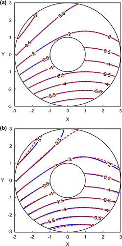
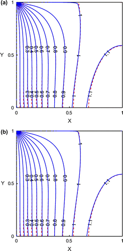
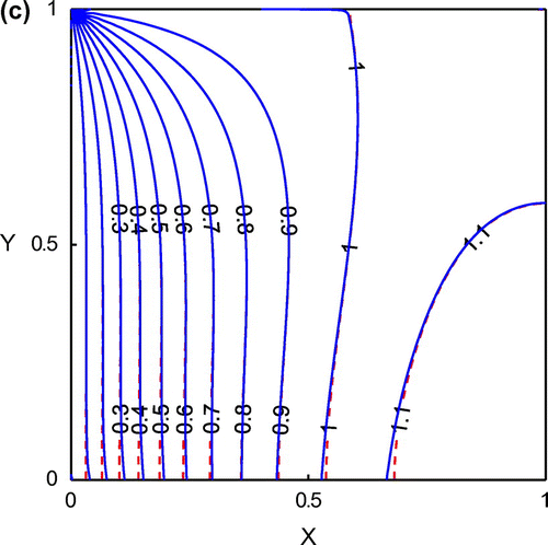
Figure 8. The distributions of numerical (solid lines) and analytical solutions (dashed lines). (a) s=0 and (b) s=3.

Figure 8. The distributions of numerical (solid lines) and analytical solutions (dashed lines). (a) s=0 and (b) s=3.

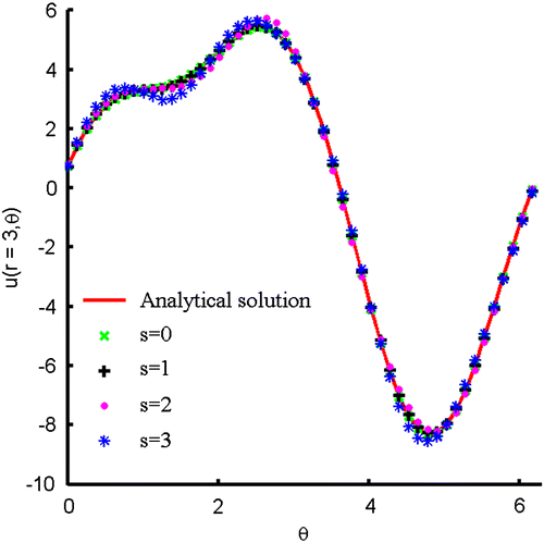
Figure 9. The profiles of numerical solutions along Γ2 for example 2.

Figure 9. The profiles of numerical solutions along Γ2 for example 2.

Table 2. The maximum absolute errors by adding different levels of noise for example 2.

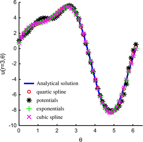
Figure 10. The profiles of numerical solutions along Γ2 by adopting different weighting functions for example 2.

Figure 10. The profiles of numerical solutions along Γ2 by adopting different weighting functions for example 2.

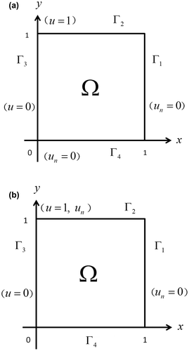
Figure 11. The schematic diagrams for example 3. (a) Direct problem and (b) inverse problem.

Figure 11. The schematic diagrams for example 3. (a) Direct problem and (b) inverse problem.

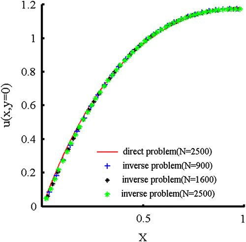
Figure 13. The profiles of numerical solutions along Γ4 for example 3.

Figure 13. The profiles of numerical solutions along Γ4 for example 3.

Reprints and Corporate Permissions

Please note: Selecting permissions does not provide access to the full text of the article, please see our help page How do I view content?

To request a reprint or corporate permissions for this article, please click on the relevant link below:

Academic Permissions

Please note: Selecting permissions does not provide access to the full text of the article, please see our help page How do I view content?

Obtain permissions instantly via Rightslink by clicking on the button below:

If you are unable to obtain permissions via Rightslink, please complete and submit this Permissions form. For more information, please visit our Permissions help page.