514
Views
14
CrossRef citations to date
0
Altmetric
Articles

Inverse shape design via a new physical-based iterative solution strategy

, &
Pages 1138-1162 | Received 18 Jan 2014, Accepted 02 Oct 2014, Published online: 07 Nov 2014

Figures & data

Figure 1. Computational grid in a curved nozzle with various control volumes and boundary conditions.
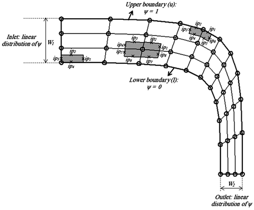
Figure 1. Computational grid in a curved nozzle with various control volumes and boundary conditions.

Figure 2. Local coordinates in a quadrilateral element.

Figure 2. Local coordinates in a quadrilateral element.

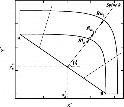
Figure 3. Spines used for grid generation.

Figure 3. Spines used for grid generation.

Figure 4. Three Solution algorithms in the context of duct design problems: (a) proposed and classical iterative algorithms (b) direct design.
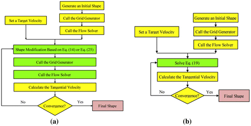
Figure 4. Three Solution algorithms in the context of duct design problems: (a) proposed and classical iterative algorithms (b) direct design.

Figure 5. Boundary control volumes in the proposed algorithm: (a) inappropriate control volumes, (b) appropriate control volumes.
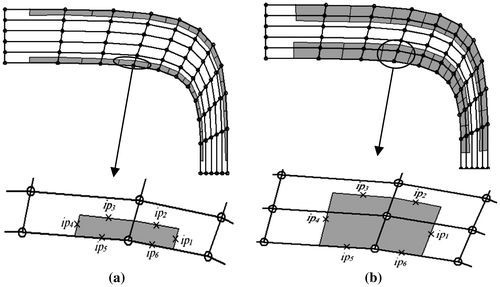
Figure 5. Boundary control volumes in the proposed algorithm: (a) inappropriate control volumes, (b) appropriate control volumes.

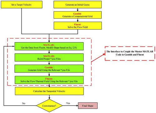
Figure 6. Iterative solution algorithm assisted with an interface to Gambit and Fluent.

Figure 6. Iterative solution algorithm assisted with an interface to Gambit and Fluent.

Figure 7. Design of a curved nozzle: (a) Initial guessed and final shape, (b) Tangential velocity for initial guessed and final shape.
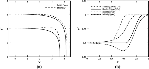
Figure 7. Design of a curved nozzle: (a) Initial guessed and final shape, (b) Tangential velocity for initial guessed and final shape.

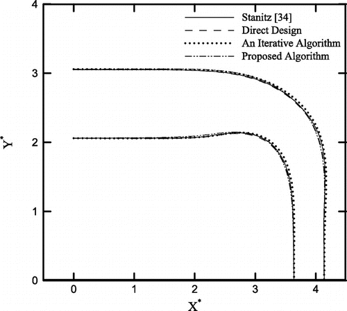
Figure 8. Design of a curved nozzle using the three different algorithms introduced in this study.

Figure 8. Design of a curved nozzle using the three different algorithms introduced in this study.

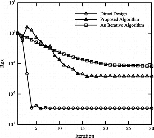
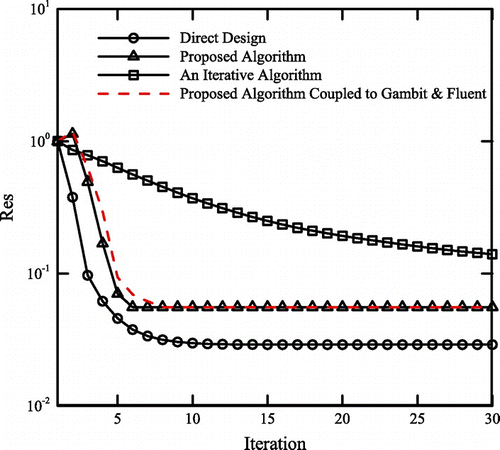
Figure 9. Convergence histories in the curved nozzle example.

Figure 9. Convergence histories in the curved nozzle example.

Figure 10. Design of a straight nozzle: (a) initial and final shapes, (b) initial and target tangential velocity distributions.
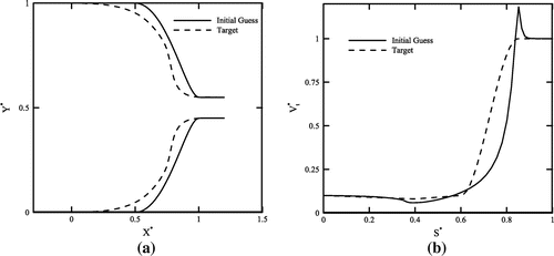
Figure 10. Design of a straight nozzle: (a) initial and final shapes, (b) initial and target tangential velocity distributions.

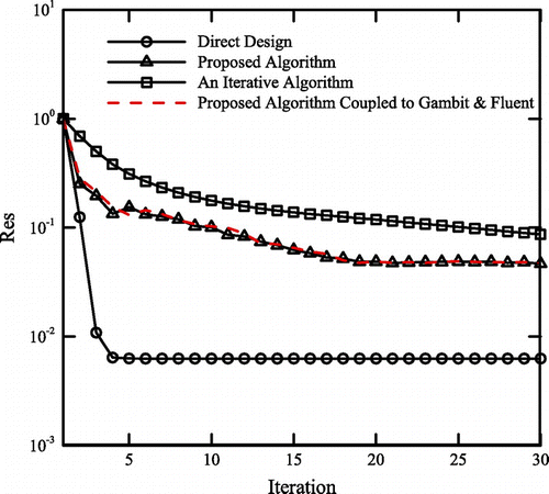
Figure 11. Convergence histories in the straight nozzle example.

Figure 11. Convergence histories in the straight nozzle example.

Figure 12. Design of a s-shaped nozzle: (a) initial and final shapes, (b) initial and target tangential velocity distributions.
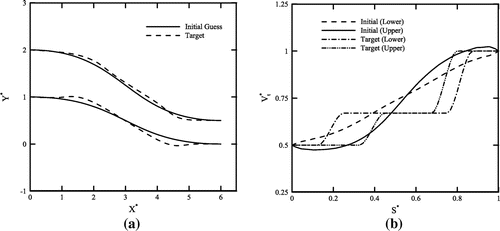
Figure 12. Design of a s-shaped nozzle: (a) initial and final shapes, (b) initial and target tangential velocity distributions.

Figure 13. Convergence histories in the s-shaped nozzle example.

Figure 13. Convergence histories in the s-shaped nozzle example.

Figure 14. Computational grid in a conducting body with various control volumes and boundary conditions.
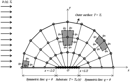
Figure 14. Computational grid in a conducting body with various control volumes and boundary conditions.

Figure 15. Design of a conducting body with uniform substrate temperature: (a) initial guess with computational grid, (b) final shapes obtained by three different algorithms introduced in this study.
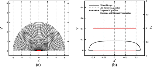
Figure 15. Design of a conducting body with uniform substrate temperature: (a) initial guess with computational grid, (b) final shapes obtained by three different algorithms introduced in this study.
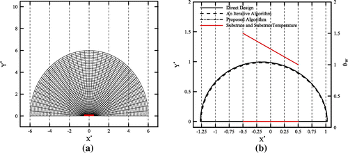
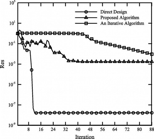
Figure 16. Convergence histories in the conducting body with uniform substrate temperature example.

Figure 16. Convergence histories in the conducting body with uniform substrate temperature example.

Figure 17. Design of a conducting body with linear substrate temperature: (a) initial guess with computational grid, (b) final shapes obtained by three different algorithms introduced in this study.
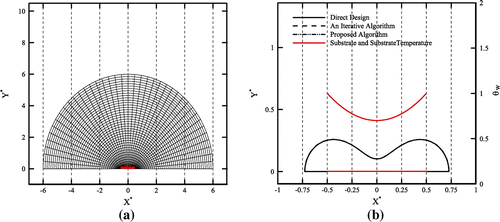
Figure 17. Design of a conducting body with linear substrate temperature: (a) initial guess with computational grid, (b) final shapes obtained by three different algorithms introduced in this study.

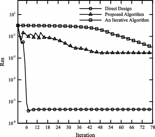
Figure 18. Convergence histories in the conducting body with linear substrate temperature example.

Figure 18. Convergence histories in the conducting body with linear substrate temperature example.

Figure 19. Design of a conducting body with nonlinear substrate temperature: (a) initial guess with computational grid, (b) final shapes obtained by three different algorithms introduced in this study.

Figure 19. Design of a conducting body with nonlinear substrate temperature: (a) initial guess with computational grid, (b) final shapes obtained by three different algorithms introduced in this study.

Figure 20. Convergence histories in the conducting body with nonlinear substrate temperature example.
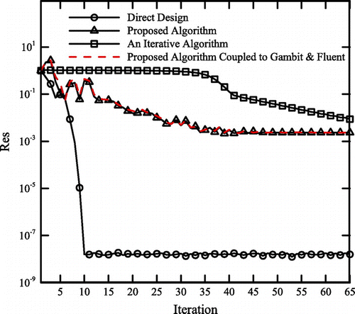
Figure 20. Convergence histories in the conducting body with nonlinear substrate temperature example.
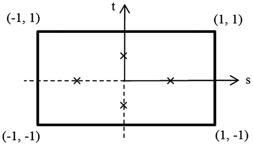
Table 1. Grid resolution, iteration number, residual level and CPU time for different test cases.

Reprints and Corporate Permissions

Please note: Selecting permissions does not provide access to the full text of the article, please see our help page How do I view content?

To request a reprint or corporate permissions for this article, please click on the relevant link below:

Academic Permissions

Please note: Selecting permissions does not provide access to the full text of the article, please see our help page How do I view content?

Obtain permissions instantly via Rightslink by clicking on the button below:

If you are unable to obtain permissions via Rightslink, please complete and submit this Permissions form. For more information, please visit our Permissions help page.