Sparsity prior for electrical impedance tomography with partial data

Figures & data

Figure 1. (a) Phantom with kite-shaped piecewise constant inclusion $\mathit{\delta }\mathit{\sigma }$. (b) Reconstruction of $\ast supp\mathit{\delta }\mathit{\sigma }$ using monotonicity relations from the approach in [45] by use of simulated noiseless data.

Figure 2. Numerical phantoms. (a) Circular piecewise constant inclusion. (b) Kite-shaped piecewise constant inclusion. (c) Multiple $C^2$ inclusions.

Figure 3. Full data sparse reconstruction of the phantoms in Figure 2 without prior information on the support of inclusions.

Figure 4. Left: Dirichlet data corresponding to $g=cos(\mathit{\theta })$ for the phantom in Figure 2(a), with 10% and 50% noise level. Middle: full data reconstruction for 10% noise level. Right: full data reconstruction for 50% noise level.

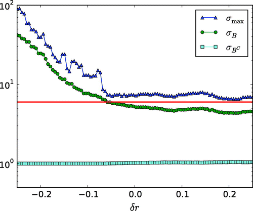
Figure 5. Full data sparse reconstruction of the phantom in Figure 2(a) varying the assumed support given by a dilation $\mathit{\delta }r$. The colour bar is truncated at $[1,6]$. For $\mathit{\delta }r<0$, the contrast in the reconstruction is higher than in the phantom.

Figure 6. Behaviour of full data sparsity reconstruction based on the phantom in Figure 2(a) by varying $\mathit{\delta }r$ characterizing the assumed support. The correct support of the inclusion is a ball $\overline{B(r^{\ast })}$ while the assumed support is $\overline{B((1+\mathit{\delta }r)r^{\ast })}$. ${\mathit{\sigma }}_B$ is the average of reconstruction $\mathit{\sigma }$ over $B(r^{\ast })$ and ${\mathit{\sigma }}_{B^C}$ is the average on the complement of $B(r^{\ast })$. ${\mathit{\sigma }}_{\text{max}}$ is the maximum of $\mathit{\sigma }$ on the mesh nodes.

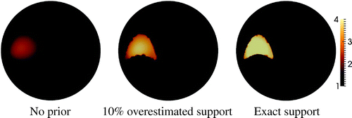
Figure 7. Full data sparse reconstruction of the phantom in Figure 2(b). The applied prior information for the overestimated support is a 10% dilation of the correct shape.

Figure 8. Sparse reconstruction of the phantom in Figure 2(c). Left: $\mathrm{\Gamma }=\mathit{\partial }\mathrm{\Omega }$. Middle: $({\mathit{\theta }}_1,{\mathit{\theta }}_2)=(0,\mathit{\pi })$. Right: $({\mathit{\theta }}_1,{\mathit{\theta }}_2)=(\mathit{\pi },2\mathit{\pi })$.

Figure 9. Sparse reconstruction of the phantom with a ball inclusion in Figure 2(a). (a) 50% boundary data, no prior. (b): 50% boundary data with 5% overestimated support. (c): 25% boundary data, no prior. (d): 25% boundary data with 5% overestimated support.

Figure 10. Sparse reconstruction of the phantom with a kite-shaped inclusion in Figure 2(b). (a) 50% boundary data, no prior. (b) 50% boundary data with 10% overestimated support. (c) 25% boundary data, no prior. (d) 25% boundary data with 10% overestimated support.

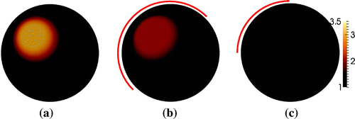
Figure 11. TV reconstruction of the phantom with a ball inclusion in Figure 2(a). (a) Full boundary data. (b) 50% boundary data. (c) 25% boundary data.

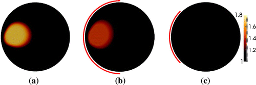
Figure 12. TV reconstruction of the phantom with a kite-shaped inclusion in Figure 2(b). (a) Full boundary data. (b) 50% boundary data. (c) 25% boundary data.

von Harrach B, Ullrich M. Monotonicity-based shape reconstruction in electrical impedance tomography. SIAM J. Math. Anal. 2013;45:3382–3403.

 Web of Science ®Google Scholar