318
Views
22
CrossRef citations to date
0
Altmetric
Articles

Migration NSGA: method to improve a non-elitist searching of Pareto front, with application in magnetics

, &
Pages 543-566 | Received 30 Jan 2015, Accepted 28 Apr 2015, Published online: 01 Jun 2015

Figures & data

Figure 1. Three different Pareto fronts and relevant starting individual sets for the same optimization problem. f1 is the magnetic field uniformity and f2 is the solution sensitivity. Both quantities are dimensionless.
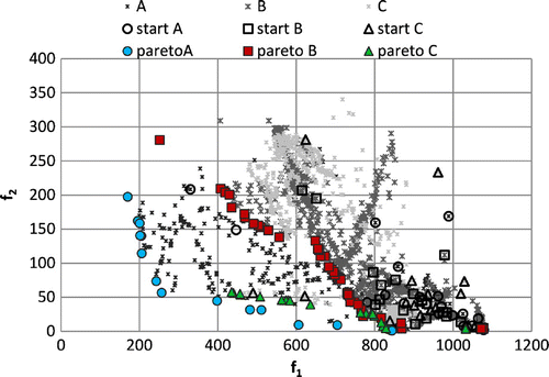
Figure 1. Three different Pareto fronts and relevant starting individual sets for the same optimization problem. f1 is the magnetic field uniformity and f2 is the solution sensitivity. Both quantities are dimensionless.

Figure 2. The flow chart of the first variant of migration NSGA algorithm: MNSGA-1; the migration occurs after the genetic operator.
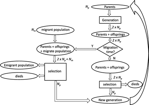
Figure 2. The flow chart of the first variant of migration NSGA algorithm: MNSGA-1; the migration occurs after the genetic operator.

Figure 3. The flow chart of the second variant of migration NSGA algorithm: M-NSGA-2; the migration occurs before the genetic operator.
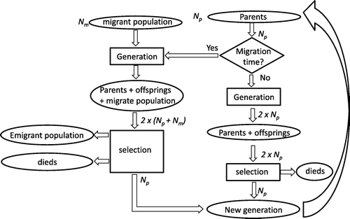
Figure 3. The flow chart of the second variant of migration NSGA algorithm: M-NSGA-2; the migration occurs before the genetic operator.

Figure 4. Test problem #1a: shape of the f1 and f2 functions in the domain.

Figure 4. Test problem #1a: shape of the f1 and f2 functions in the domain.

Figure 5. Test problem #1: (a) and (c) analytical Pareto front and (b) and (d) analytical inverse image of Pareto front for problem #1a and #1b, respectively.
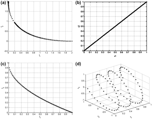
Figure 5. Test problem #1: (a) and (c) analytical Pareto front and (b) and (d) analytical inverse image of Pareto front for problem #1a and #1b, respectively.

Figure 6. (a) Geometry of the device with eight design variables and three uncertain parameters (parameters underlined). (b) Mesh detail.
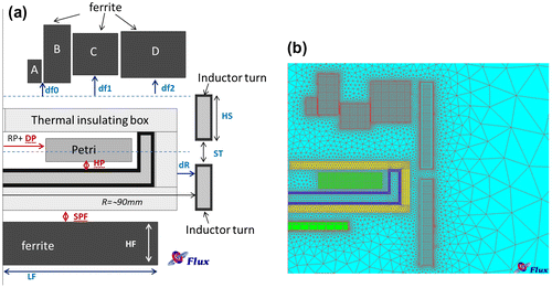
Figure 6. (a) Geometry of the device with eight design variables and three uncertain parameters (parameters underlined). (b) Mesh detail.

Figure 7. (a) Pareto front and (b) design variable space representation obtained using NSGA-II algorithm considering a population of Np = 20 individuals, Ng = 20 generations and three different initial sets of design variables. (c) Pareto front and (d) design variable space representation obtained using NSGA-II algorithm considering Np = 50 individuals, Ng = 20 generations and three different initial sets of design variables.
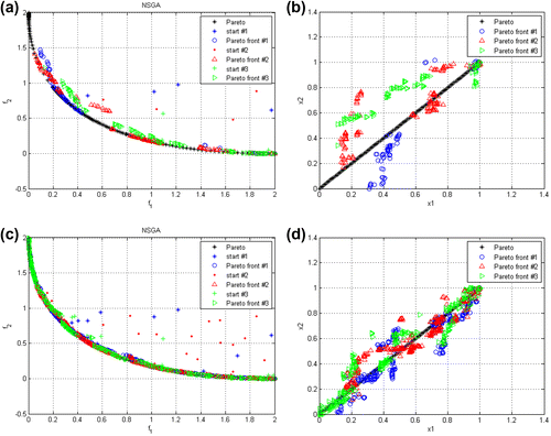
Figure 7. (a) Pareto front and (b) design variable space representation obtained using NSGA-II algorithm considering a population of Np = 20 individuals, Ng = 20 generations and three different initial sets of design variables. (c) Pareto front and (d) design variable space representation obtained using NSGA-II algorithm considering Np = 50 individuals, Ng = 20 generations and three different initial sets of design variables.

Figure 8. Comparison of (a) the Pareto front obtained using classical NSGA-II, MNSGA-1 and MNSGA-2 algorithm considering Ng = 20, Np = 20, Nm = 10, and Tm = 5. (b) Comparison of the design variable space obtained using classical NSGA-II, MNSGA-1 and MNSGA-2 algorithms. Crowding distance on (c) objective space and (d) on design variable space.
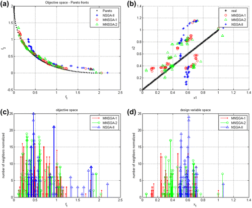
Figure 8. Comparison of (a) the Pareto front obtained using classical NSGA-II, MNSGA-1 and MNSGA-2 algorithm considering Ng = 20, Np = 20, Nm = 10, and Tm = 5. (b) Comparison of the design variable space obtained using classical NSGA-II, MNSGA-1 and MNSGA-2 algorithms. Crowding distance on (c) objective space and (d) on design variable space.
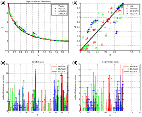
Figure 9. Comparison of (a) the Pareto front obtained using classical NSGA-II, MNSGA-1 and MNSGA-2 algorithm considering Ng = 20, Np = 20, Nm = 20, and Tm = 5. (b) Comparison of the design variable space obtained using classical NSGA-II, MNSGA-1 and MNSGA-2 algorithms. Crowding distance on (c) objective space and (d) on design variable space.
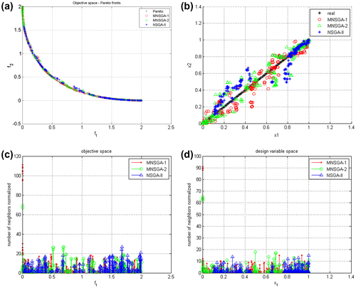
Figure 9. Comparison of (a) the Pareto front obtained using classical NSGA-II, MNSGA-1 and MNSGA-2 algorithm considering Ng = 20, Np = 20, Nm = 20, and Tm = 5. (b) Comparison of the design variable space obtained using classical NSGA-II, MNSGA-1 and MNSGA-2 algorithms. Crowding distance on (c) objective space and (d) on design variable space.

Figure 10. Comparison of (a) the Pareto front obtained using classical NSGA-II, MNSGA-1 and MNSGA-2 algorithm considering Ng = 50, Np = 20, Nm = 10, and Tm = 2. (b) Comparison of the design variable space obtained using classical NSGA-II, MNSGA-1 and MNSGA-2 algorithms. Crowding distance on (c) objective space and (d) on design variable space.

Figure 10. Comparison of (a) the Pareto front obtained using classical NSGA-II, MNSGA-1 and MNSGA-2 algorithm considering Ng = 50, Np = 20, Nm = 10, and Tm = 2. (b) Comparison of the design variable space obtained using classical NSGA-II, MNSGA-1 and MNSGA-2 algorithms. Crowding distance on (c) objective space and (d) on design variable space.

Figure 11. Comparison of the Pareto front and the design variable space obtained using classical NSGA-II, MNSGA-1 and MNSGA-2 algorithm considering Ng = 20, Np = 20, Nm = 10 (a) and (e) Tm = 2 and (b) and (f) Tm = 5. Crowding distance on (c) and (g) objective space and (d) and (h) on design variable space for Tm = 2 and 5, respectively.
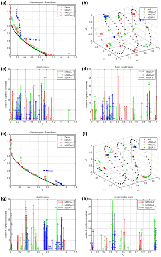
Figure 11. Comparison of the Pareto front and the design variable space obtained using classical NSGA-II, MNSGA-1 and MNSGA-2 algorithm considering Ng = 20, Np = 20, Nm = 10 (a) and (e) Tm = 2 and (b) and (f) Tm = 5. Crowding distance on (c) and (g) objective space and (d) and (h) on design variable space for Tm = 2 and 5, respectively.

Table 1. Results of the tests performed: average of the rms error evaluated on inverse image using (19) and objective space using (20) of 30 optimization runs.

Table 2. Results of the T-test (p-value) in order to compare rms error data resumed in Table of MNSGA-1 and NSGA-II, MNSGA-2 and NSGA-II, and MNSGA-1 and MNSGA-2.

Figure 12. (a) The approximated Pareto front using classical NSGA-II algorithm with Np = 50 and Ng = 50, (b) the BH curves estimated using design variables of solutions in the Pareto set, (c) the approximated Pareto front using classical NSGA-II algorithm with Np = 20 and Ng = 50 and (d) the BH curves estimated using design variables of solutions in the Pareto set.

Figure 12. (a) The approximated Pareto front using classical NSGA-II algorithm with Np = 50 and Ng = 50, (b) the B–H curves estimated using design variables of solutions in the Pareto set, (c) the approximated Pareto front using classical NSGA-II algorithm with Np = 20 and Ng = 50 and (d) the B–H curves estimated using design variables of solutions in the Pareto set.
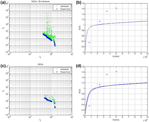
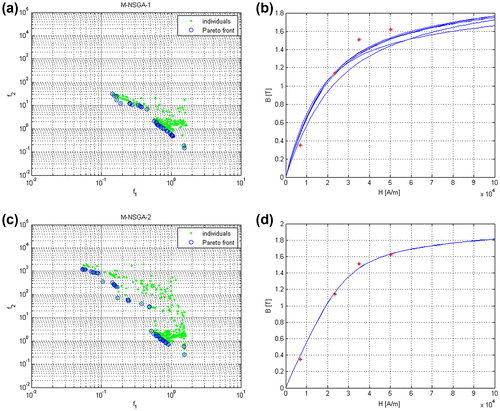
Figure 13. The approximated Pareto front using (a) MNSGA-1 and (c) MNSGA-2. Algorithms setting Np = 20, Ng = 50, Nm = 10 and Tm = 5. (b) and (d) are the BH curves estimated using design variables of solutions in the Pareto set.

Figure 13. The approximated Pareto front using (a) MNSGA-1 and (c) MNSGA-2. Algorithms setting Np = 20, Ng = 50, Nm = 10 and Tm = 5. (b) and (d) are the B–H curves estimated using design variables of solutions in the Pareto set.
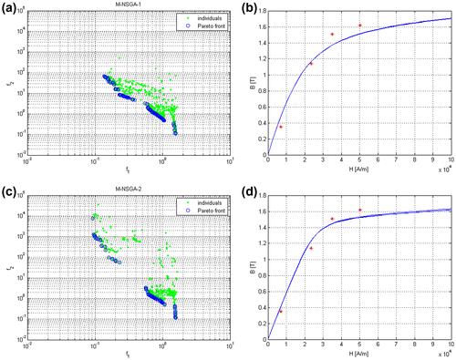
Figure 14. (a) The approximated Pareto front using (a) MNSGA-1 and (c) MNSGA-2. Algorithms setting Np = 20, Ng = 20, Nm = 10 and Tm = 2. (b) and (d) are the BH curves estimated using design variables of solutions in the Pareto set.

Figure 14. (a) The approximated Pareto front using (a) MNSGA-1 and (c) MNSGA-2. Algorithms setting Np = 20, Ng = 20, Nm = 10 and Tm = 2. (b) and (d) are the B–H curves estimated using design variables of solutions in the Pareto set.
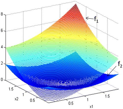
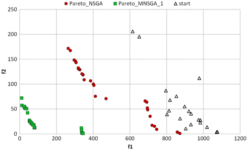
Figure 15. Approximated Pareto front using NSGA-II (circles) and MNSGA-1 (squares) algorithm starting from the same initial population (triangles) for the problem #3.

Figure 15. Approximated Pareto front using NSGA-II (circles) and MNSGA-1 (squares) algorithm starting from the same initial population (triangles) for the problem #3.

Reprints and Corporate Permissions

Please note: Selecting permissions does not provide access to the full text of the article, please see our help page How do I view content?

To request a reprint or corporate permissions for this article, please click on the relevant link below:

Academic Permissions

Please note: Selecting permissions does not provide access to the full text of the article, please see our help page How do I view content?

Obtain permissions instantly via Rightslink by clicking on the button below:

If you are unable to obtain permissions via Rightslink, please complete and submit this Permissions form. For more information, please visit our Permissions help page.