407
Views
0
CrossRef citations to date
0
Altmetric
Articles

Reconstruction of multiplicative space- and time-dependent sources

&
Pages 1528-1549 | Received 22 Apr 2015, Accepted 07 Dec 2015, Published online: 12 Jan 2016

Figures & data

Table 1. The RMSE (Equation5.1) and (Equation5.2) for u(0,t),u(0.1,t),β(t) and μ(x), obtained using the BEM for the direct problem with N=N0{10,20,40}, for Example 1.

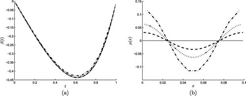
Figure 1. The analytical (—–) and numerical results for (a) β(t) and (b) μ(x) obtained using the BEM for the direct problem with N=N0{10(-·-),20(),40(---)}, for Example 1.

Figure 1. The analytical (—–) and numerical results for (a) β(t) and (b) μ(x) obtained using the BEM for the direct problem with N=N0∈{10(-·-),20(⋯),40(---)}, for Example 1.

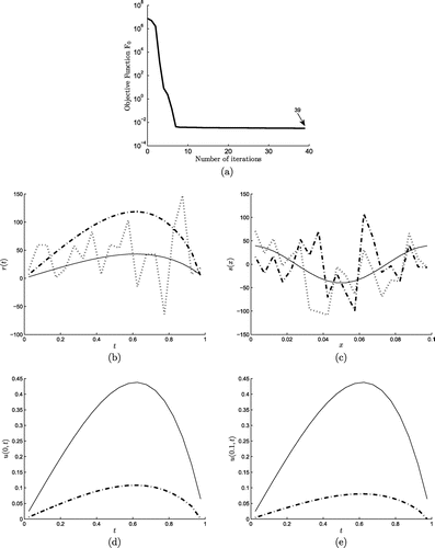
Figure 2. (a) The objective function F0 and the numerical results for (b) r(t), (c) s(x), (d) u(0, t), (e) u(0.1, t) obtained with no regularization (-·-), for exact data for Example 1. The corresponding analytical solutions are shown by continuous line (—–) in (b)–(e) and the p0=100% perturbed initial guesses are shown by dotted line () in (b) and (c).

Figure 2. (a) The objective function F0 and the numerical results for (b) r(t), (c) s(x), (d) u(0, t), (e) u(0.1, t) obtained with no regularization (-·-), for exact data for Example 1. The corresponding analytical solutions are shown by continuous line (—–) in (b)–(e) and the p0=100% perturbed initial guesses are shown by dotted line (⋯) in (b) and (c).

Figure 3. The numerical results for (a) r(t), (b) s(x), (c) u(0, t), (d) u(0.1, t) obtained with the first-order regularization () and the second-order regularization (---) with regularization parameter λ=10-5, for exact data for Example 1. The corresponding analytical solutions are shown by continuous line (—–).
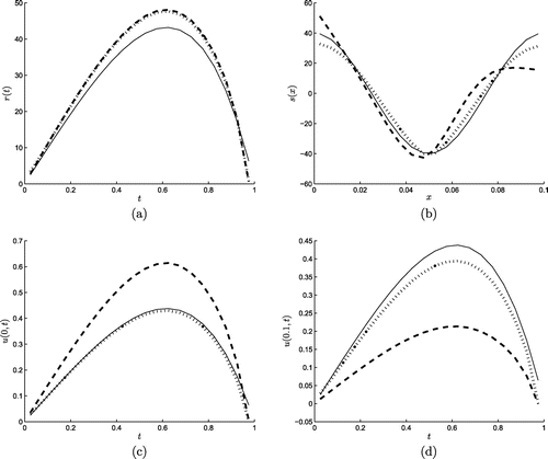
Figure 3. The numerical results for (a) r(t), (b) s(x), (c) u(0, t), (d) u(0.1, t) obtained with the first-order regularization (⋯) and the second-order regularization (---) with regularization parameter λ=10-5, for exact data for Example 1. The corresponding analytical solutions are shown by continuous line (—–).

Table 2. The RMSE (Equation5.1) and (Equation5.2) for r(t),s(x),u(0,t),u(0.1,t) for exact data for Example 1.

Figure 4. (a) The L-curve criterion, (b) the objective function Fλ, and the numerical results (--)for (c) r(t), (d) s(x), (e) u(0, t), (f) u(0.1, t) obtained with the hybrid-order regularization (Equation5.12) with regularization parameter λ=10-5 suggested by L-curve, for exact data for Example 1. The corresponding analytical solutions are shown by continuous line (—–) in (c)–(f).
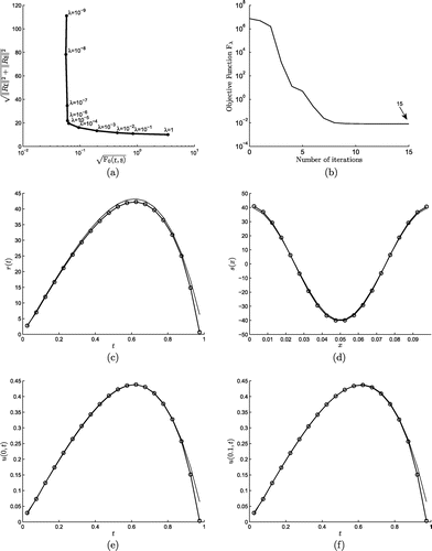
Figure 4. (a) The L-curve criterion, (b) the objective function Fλ, and the numerical results (-∘-)for (c) r(t), (d) s(x), (e) u(0, t), (f) u(0.1, t) obtained with the hybrid-order regularization (Equation5.12(5.12) Fλ(r̲,s̲)=F0(r̲,s̲)+λ((r1-r2)2+(-rN-1+rN)2+∑i=2N-1(-ri+1+2ri-ri-1)2+(s1-s2)2+(-sN0-1+sN0)2+∑k=2N0-1(-sk+1+2sk-sk-1)2).(5.12) ) with regularization parameter λ=10-5 suggested by L-curve, for exact data for Example 1. The corresponding analytical solutions are shown by continuous line (—–) in (c)–(f).

Figure 5. (a) The objective function Fλ and the numerical results for (b) r(t), (c) s(x), (d) u(0, t), (e) u(0.1, t) obtained with the hybrid-order regularization (Equation5.12) with regularization parameter λ=10-5 for P{1(-·-),3(),5(---)}% noisy data for Example 1. The corresponding analytical solutions are shown by continuous line (—–) in (b)–(e).
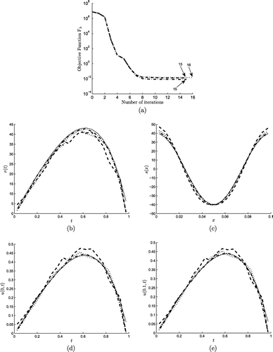
Figure 5. (a) The objective function Fλ and the numerical results for (b) r(t), (c) s(x), (d) u(0, t), (e) u(0.1, t) obtained with the hybrid-order regularization (Equation5.12(5.12) Fλ(r̲,s̲)=F0(r̲,s̲)+λ((r1-r2)2+(-rN-1+rN)2+∑i=2N-1(-ri+1+2ri-ri-1)2+(s1-s2)2+(-sN0-1+sN0)2+∑k=2N0-1(-sk+1+2sk-sk-1)2).(5.12) ) with regularization parameter λ=10-5 for P∈{1(-·-),3(⋯),5(---)}% noisy data for Example 1. The corresponding analytical solutions are shown by continuous line (—–) in (b)–(e).

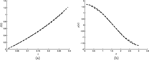
Figure 6. The analytical (—–) and numerical results for (a) β(t) and (b) μ(x) obtained using the BEM for the direct problem with N=N0{5(-·-),10(),20(---)}, for Example 2.

Figure 6. The analytical (—–) and numerical results for (a) β(t) and (b) μ(x) obtained using the BEM for the direct problem with N=N0∈{5(-·-),10(⋯),20(---)}, for Example 2.

Table 3. The RMSEs (Equation5.1) and (Equation5.2) for r(t) and s(x), for the noise levels δ{0,0.01,0.1}, for Example 2.

Figure 7. (a) The objective function F0, (b) the RMSEs (Equation5.1) and (Equation5.2) for r(t)(---) and s(x)() obtained with no regularization for exact data, and the numerical results for (c) r(t) and (d) s(x) obtained using the minimization process after 56 unfixed iterations (-·-), and 31 fixed iterations (), for Example 2. The corresponding analytical solutions (Equation5.18) are shown by continuous line (—–) in (c) and (d).
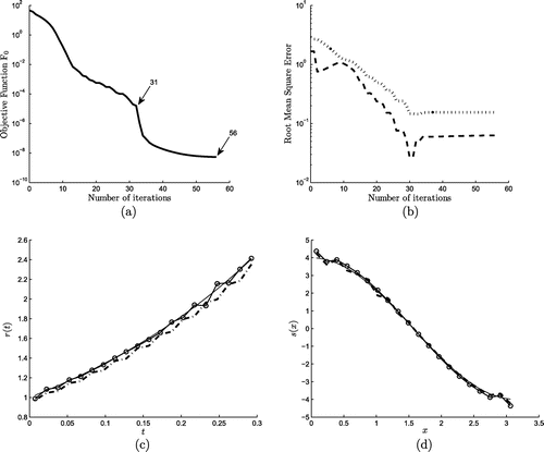
Figure 7. (a) The objective function F0, (b) the RMSEs (Equation5.1(5.1) RMSEt=1N∑i=1NExact(t~i)-Numerical(t~i)2,(5.1) ) and (Equation5.2(5.2) RMSEx=1N0∑k=1N0Exact(x~k)-Numerical(x~k)2.(5.2) ) for r(t)(---) and s(x)(⋯) obtained with no regularization for exact data, and the numerical results for (c) r(t) and (d) s(x) obtained using the minimization process after 56 unfixed iterations (-·-), and 31 fixed iterations (∘∘∘), for Example 2. The corresponding analytical solutions (Equation5.18(5.18) r(t)=e3t,s(x)=4cos(x),t∈(0,0.3),x∈(0,π),(5.18) ) are shown by continuous line (—–) in (c) and (d).
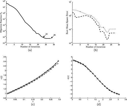
Figure 8. (a) The objective function Fλ, (b) the RMSEs (Equation5.1) and (Equation5.2) for r(t)(---) and s(x)() obtained using the hybrid-order regularization (Equation5.12) with regularization parameter λ=2×10⁻⁴ for exact data, and the numerical results for (c) r(t) and (d) s(x) obtained using minimization process after 28 unfixed iterations (-·-), and 23 fixed iterations (), for Example 2. The corresponding analytical solutions (Equation5.18) are shown by continuous line (—–) in (c) and (d).
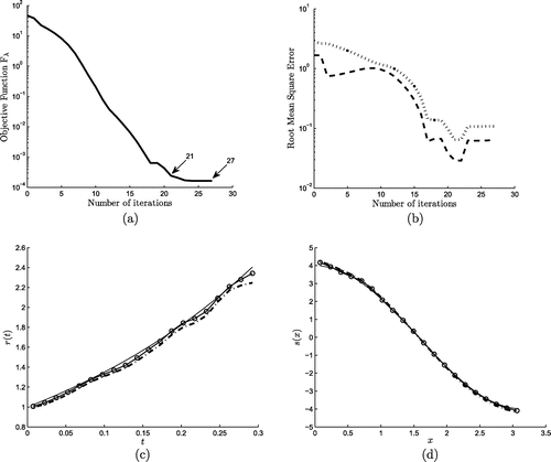
Figure 8. (a) The objective function Fλ, (b) the RMSEs (Equation5.1(5.1) RMSEt=1N∑i=1NExact(t~i)-Numerical(t~i)2,(5.1) ) and (Equation5.2(5.2) RMSEx=1N0∑k=1N0Exact(x~k)-Numerical(x~k)2.(5.2) ) for r(t)(---) and s(x)(⋯) obtained using the hybrid-order regularization (Equation5.12(5.12) Fλ(r̲,s̲)=F0(r̲,s̲)+λ((r1-r2)2+(-rN-1+rN)2+∑i=2N-1(-ri+1+2ri-ri-1)2+(s1-s2)2+(-sN0-1+sN0)2+∑k=2N0-1(-sk+1+2sk-sk-1)2).(5.12) ) with regularization parameter λ=2×10⁻⁴ for exact data, and the numerical results for (c) r(t) and (d) s(x) obtained using minimization process after 28 unfixed iterations (-·-), and 23 fixed iterations (∘∘∘), for Example 2. The corresponding analytical solutions (Equation5.18(5.18) r(t)=e3t,s(x)=4cos(x),t∈(0,0.3),x∈(0,π),(5.18) ) are shown by continuous line (—–) in (c) and (d).
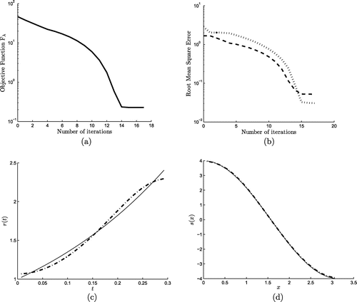
Figure 9. (a) The objective function Fλ, (b) the RMSEs (Equation5.1) and (Equation5.2) for r(t)(---) and s(x)() obtained using the hybrid-order regularization (Equation5.12) with regularization parameter λ=4×10⁻⁴ for noise level δ=0.01, and the numerical results for (c) r(t) and (d) s(x) obtained using the minimization process after 27 unfixed iterations (-·-), and 21 fixed iterations (), for Example 2. The corresponding analytical solutions (Equation5.18) are shown by continuous line (—–) in (c) and (d).

Figure 9. (a) The objective function Fλ, (b) the RMSEs (Equation5.1(5.1) RMSEt=1N∑i=1NExact(t~i)-Numerical(t~i)2,(5.1) ) and (Equation5.2(5.2) RMSEx=1N0∑k=1N0Exact(x~k)-Numerical(x~k)2.(5.2) ) for r(t)(---) and s(x)(⋯) obtained using the hybrid-order regularization (Equation5.12(5.12) Fλ(r̲,s̲)=F0(r̲,s̲)+λ((r1-r2)2+(-rN-1+rN)2+∑i=2N-1(-ri+1+2ri-ri-1)2+(s1-s2)2+(-sN0-1+sN0)2+∑k=2N0-1(-sk+1+2sk-sk-1)2).(5.12) ) with regularization parameter λ=4×10⁻⁴ for noise level δ=0.01, and the numerical results for (c) r(t) and (d) s(x) obtained using the minimization process after 27 unfixed iterations (-·-), and 21 fixed iterations (∘∘∘), for Example 2. The corresponding analytical solutions (Equation5.18(5.18) r(t)=e3t,s(x)=4cos(x),t∈(0,0.3),x∈(0,π),(5.18) ) are shown by continuous line (—–) in (c) and (d).

Figure 10. (a) The objective function Fλ, (b) the RMSEs (Equation5.1) and (Equation5.2) for r(t)(---) and s(x)() obtained using the hybrid-order regularization (Equation5.12) with regularization parameter λ=2 for noise level δ=0.1, and the numerical results (-·-) for (c) r(t) and (d) s(x) obtained using the minimization process after 17 (unfixed) iterations, for Example 2. The corresponding analytical solutions (Equation5.18) are shown by continuous line (—–) in (c) and (d).

Figure 10. (a) The objective function Fλ, (b) the RMSEs (Equation5.1(5.1) RMSEt=1N∑i=1NExact(t~i)-Numerical(t~i)2,(5.1) ) and (Equation5.2(5.2) RMSEx=1N0∑k=1N0Exact(x~k)-Numerical(x~k)2.(5.2) ) for r(t)(---) and s(x)(⋯) obtained using the hybrid-order regularization (Equation5.12(5.12) Fλ(r̲,s̲)=F0(r̲,s̲)+λ((r1-r2)2+(-rN-1+rN)2+∑i=2N-1(-ri+1+2ri-ri-1)2+(s1-s2)2+(-sN0-1+sN0)2+∑k=2N0-1(-sk+1+2sk-sk-1)2).(5.12) ) with regularization parameter λ=2 for noise level δ=0.1, and the numerical results (-·-) for (c) r(t) and (d) s(x) obtained using the minimization process after 17 (unfixed) iterations, for Example 2. The corresponding analytical solutions (Equation5.18(5.18) r(t)=e3t,s(x)=4cos(x),t∈(0,0.3),x∈(0,π),(5.18) ) are shown by continuous line (—–) in (c) and (d).

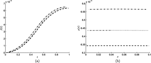
Figure 11. The numerical results for (a) β(t) and (b) μ(x) obtained using the BEM for the direct problem with N=N0{10(-·-),20(),40(---)}, for Example 3.

Figure 11. The numerical results for (a) β(t) and (b) μ(x) obtained using the BEM for the direct problem with N=N0∈{10(-·-),20(⋯),40(---)}, for Example 3.

Figure 12. (a) The objective function Fλ and the numerical results for (b) r(t) and (c) s(x) obtained with the hybrid-order regularization (Equation5.12) with regularization parameter λ=2×10⁻⁴ for P=1%(-·-),P=5%() and P=10%(---) noisy data for Example 3. The corresponding analytical solutions (Equation5.21) are shown by continuous line (—–) in (b) and (c).
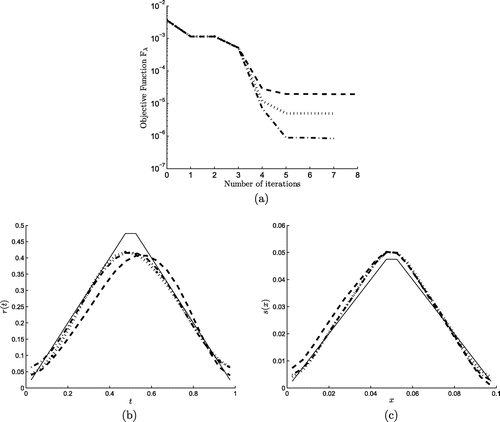
Figure 12. (a) The objective function Fλ and the numerical results for (b) r(t) and (c) s(x) obtained with the hybrid-order regularization (Equation5.12(5.12) Fλ(r̲,s̲)=F0(r̲,s̲)+λ((r1-r2)2+(-rN-1+rN)2+∑i=2N-1(-ri+1+2ri-ri-1)2+(s1-s2)2+(-sN0-1+sN0)2+∑k=2N0-1(-sk+1+2sk-sk-1)2).(5.12) ) with regularization parameter λ=2×10⁻⁴ for P=1%(-·-),P=5%(⋯) and P=10%(---) noisy data for Example 3. The corresponding analytical solutions (Equation5.21(5.21) r(t)=t,0≤t≤1/21-t,1/2<t≤1=T,s(x)=x,0≤x≤1/200.1-x,1/20<x≤1/10=L,(5.21) ) are shown by continuous line (—–) in (b) and (c).

Reprints and Corporate Permissions

Please note: Selecting permissions does not provide access to the full text of the article, please see our help page How do I view content?

To request a reprint or corporate permissions for this article, please click on the relevant link below:

Academic Permissions

Please note: Selecting permissions does not provide access to the full text of the article, please see our help page How do I view content?

Obtain permissions instantly via Rightslink by clicking on the button below:

If you are unable to obtain permissions via Rightslink, please complete and submit this Permissions form. For more information, please visit our Permissions help page.