A Gaussian RBFs method with regularization for the numerical solution of inverse heat conduction problems

Figures & data

Figure 1. The plots of RMS(c) with respect to c for two classes of initial condition of Example 1: (a) The global initial condition case, (b) The partial initial condition case.

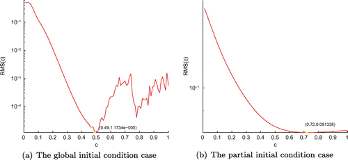
Figure 2. The plots of the exact function u(x, 0) and its approximation (a) with four different noise levels added to the measured data, namely $\mathit{\delta }=0.01\%,\mathit{\delta }=0.1\%,\mathit{\delta }=1\%$ and $\mathit{\delta }=5\%$ for the partial initial condition case, and RMS($\tilde{n}$) (b) with respect to the integer $\tilde{n}$ of Example 1.

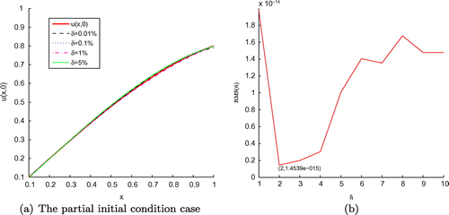
Figure 3. The RMS error (a) of function u(x, t) and its maximum error (b) with $T=1$, and four different noise levels added to the measured data, namely $\mathit{\delta }=0.01\%,\mathit{\delta }=0.1\%,\mathit{\delta }=1\%$ and $\mathit{\delta }=5\%$, for the global initial condition case of Example 1, L denotes time level corresponding to $t=0,0.1,\dots ,1$.

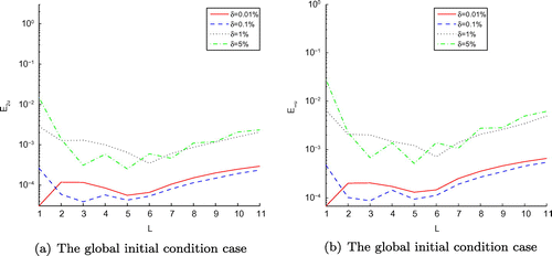
Table 1. The results of $E_{2f}$, $E_{\infty f}$, ${\mathit{\alpha }}_{\text{opt}}(A_0)$ and ${\mathit{\alpha }}_{\text{opt}}(B_0)$ with various error levels, namely $\mathit{\delta }=0.01\%,\mathit{\delta }=0.1\%,\mathit{\delta }=1\%$ and $\mathit{\delta }=5\%$ for the global initial condition case of Example 1.

	$\mathit{\delta }=0.01\%$	$\mathit{\delta }=0.1\%$	$\mathit{\delta }=1\%$	$\mathit{\delta }=5\%$
$E_{2f}$	$8.57\times {10}^{-4}$	$1.25\times {10}^{-3}$	$6.98\times {10}^{-3}$	$8.83\times {10}^{-3}$
$E_{\infty f}$	$1.56\times {10}^{-3}$	$3.01\times {10}^{-3}$	$1.24\times {10}^{-2}$	$1.85\times {10}^{-2}$
${\mathit{\alpha }}_{\text{opt}}(A_0)$	$0.30\times {10}^{-9}$	$0.30\times {10}^{-10}$	$0.30\times {10}^{-6}$	$0.30\times {10}^{-6}$
${\mathit{\alpha }}_{\text{opt}}(B_0)$	$0.80\times {10}^{-9}$	$0.30\times {10}^{-10}$	$0.80\times {10}^{-7}$	$0.80\times {10}^{-8}$

Figure 4. The RMS error (a) of function u(x, t) and its maximum error (b) with $T=1$, and four different noise levels added to the measured data, namely $\mathit{\delta }=0.01\%,\mathit{\delta }=0.1\%,\mathit{\delta }=1\%$ and $\mathit{\delta }=5\%$, for the partial initial condition case of Example 1, L denotes time level corresponding to $t=0,0.1,\dots ,1$.

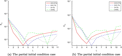
Figure 5. The exact function f(t) and its approximation with four different noise levels added to the measured data, where $\mathit{\delta }=0.01\%,\mathit{\delta }=0.1\%,\mathit{\delta }=1\%$ and $\mathit{\delta }=5\%$ for the global (a) and partial (b) initial condition cases of Example 1.

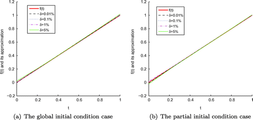
Table 2. The results of $E_{2f}$, $E_{\infty f}$, $E_{2h_2}$, $E_{\infty h_2}$, ${\mathit{\alpha }}_{\text{opt}}(A_0)$ and ${\mathit{\alpha }}_{\text{opt}}(C_0)$ with various error levels, namely $\mathit{\delta }=0.01\%,\mathit{\delta }=0.1\%,\mathit{\delta }=1\%$ and $\mathit{\delta }=5\%$ for the partial initial condition case of Example 1.

	$\mathit{\delta }=0.01\%$	$\mathit{\delta }=0.1\%$	$\mathit{\delta }=1\%$	$\mathit{\delta }=5\%$
$E_{2f}$	$1.69\times {10}^{-3}$	$5.14\times {10}^{-3}$	$4.83\times {10}^{-3}$	$6.43\times {10}^{-3}$
$E_{\infty f}$	$6.07\times {10}^{-3}$	$1.81\times {10}^{-2}$	$1.61\times {10}^{-2}$	$2.00\times {10}^{-2}$
$E_{2h_2}$	$3.52\times {10}^{-3}$	$4.23\times {10}^{-3}$	$3.13\times {10}^{-3}$	$4.89\times {10}^{-3}$
$E_{\infty h_2}$	$8.94\times {10}^{-3}$	$8.40\times {10}^{-3}$	$6.01\times {10}^{-3}$	$8.35\times {10}^{-3}$
${\mathit{\alpha }}_{\text{opt}}(A_0)$	$0.30\times {10}^{-8}$	$0.50\times {10}^{-9}$	$0.50\times {10}^{-10}$	$0.80\times {10}^{-11}$
${\mathit{\alpha }}_{\text{opt}}(C_0)$	$0.90\times {10}^{-6}$	$1.10\times {10}^{-6}$	$0.85\times {10}^{-4}$	$0.22\times {10}^{-3}$

Figure 6. The plots of RMS(c) with respect to c for two classes of initial condition of Example 2: (a) The global initial condition case, (b) The partial initial condition case.

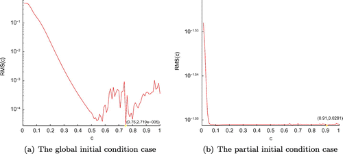
Figure 7. The plots of the exact function u(x, 0) and its approximation (a) with four different noise levels added to the measured data, namely $\mathit{\delta }=0.02\%,\mathit{\delta }=0.2\%,\mathit{\delta }=1\%$ and $\mathit{\delta }=5\%$ for the partial initial condition case, and RMS($\tilde{n}$) (b) with respect to the integer $\tilde{n}$ of Example 2.

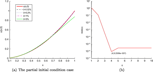
Figure 8. The plots of the exact f(t) and its approximation function to see literature [15] in Example 2.

Figure 9. The exact function f(t) and its approximation with four different noise levels added to the measured data, namely $\mathit{\delta }=0.01\%,\mathit{\delta }=0.1\%,\mathit{\delta }=1\%$ and $\mathit{\delta }=5\%$ for the global (a) initial condition case of Example 2 , and the partial (b) initial condition case with $\mathit{\delta }=0.02\%,\mathit{\delta }=0.2\%,\mathit{\delta }=1\%$ and $\mathit{\delta }=5\%$, respectively.

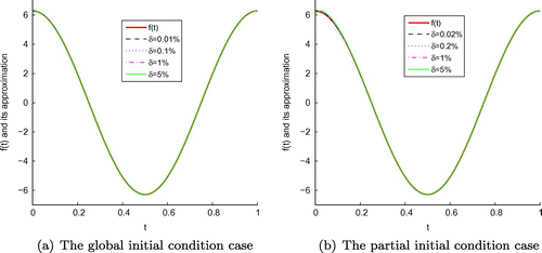
Table 3. The results of $E_{2f}$, $E_{\infty f}$, ${\mathit{\alpha }}_{\text{opt}}(A_0)$ and ${\mathit{\alpha }}_{\text{opt}}(B_0)$ with various error levels, $\mathit{\delta }=0.01\%,\mathit{\delta }=0.1\%,\mathit{\delta }=1\%$ and $\mathit{\delta }=5\%$ for the global initial condition case of Example 2.

	$\mathit{\delta }=0.01\%$	$\mathit{\delta }=0.1\%$	$\mathit{\delta }=1\%$	$\mathit{\delta }=5\%$
$E_{2f}$	$1.74\times {10}^{-3}$	$1.81\times {10}^{-3}$	$7.09\times {10}^{-3}$	$9.89\times {10}^{-3}$
$E_{\infty f}$	$1.18\times {10}^{-2}$	$1.43\times {10}^{-2}$	$5.28\times {10}^{-2}$	$8.85\times {10}^{-2}$
${\mathit{\alpha }}_{\text{opt}}(A_0)$	$0.30\times {10}^{-9}$	$0.30\times {10}^{-9}$	$0.30\times {10}^{-10}$	$0.50\times {10}^{-9}$
${\mathit{\alpha }}_{\text{opt}}(B_0)$	$0.40\times {10}^{-10}$	$0.30\times {10}^{-9}$	$0.30\times {10}^{-10}$	$0.30\times {10}^{-9}$

Figure 10. The RMS error (a) of function u(x, t) and its maximum error (b) with $T=1$, and four noise levels added to the measured data, namely $\mathit{\delta }=0.01\%,\mathit{\delta }=0.1\%,\mathit{\delta }=1\%$ and $\mathit{\delta }=5\%$, for the global initial condition case of Example 2, L denotes time level corresponding to $t=0,0.1,\dots ,1$.

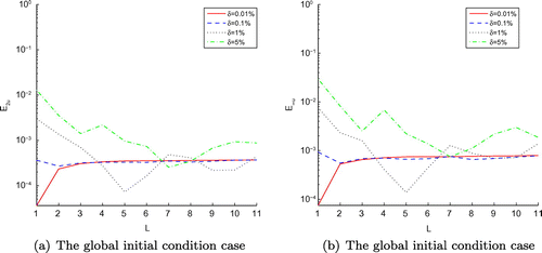
Figure 11. The RMS error (a) of function u(x, t) and its maximum error (b) with $T=1$, with four different noise levels added to the measured data, namely $\mathit{\delta }=0.02\%,\mathit{\delta }=0.2\%,\mathit{\delta }=1\%$ and $\mathit{\delta }=5\%$, for the partial initial condition case of Example 2, L denotes time level corresponding to $t=0,0.1,\dots ,1$.

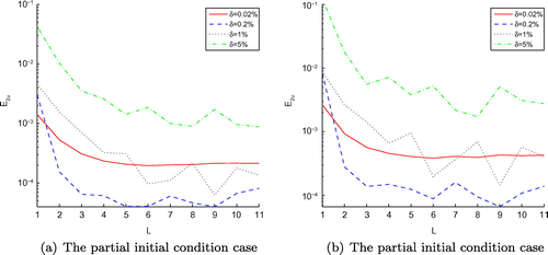
Table 4. The results of $E_{2f}$, $E_{\infty f}$, $E_{2h_2}$, $E_{\infty h_2}$, ${\mathit{\alpha }}_{\text{opt}}(A_0)$ and ${\mathit{\alpha }}_{\text{opt}}(C_0)$ with various error levels, namely $\mathit{\delta }=0.02\%,\mathit{\delta }=0.2\%,\mathit{\delta }=1\%$ and $\mathit{\delta }=5\%$ for the partial initial condition case of Example 2.

	$\mathit{\delta }=0.02\%$	$\mathit{\delta }=0.2\%$	$\mathit{\delta }=1\%$	$\mathit{\delta }=5\%$
$E_{2f}$	$3.64\times {10}^{-3}$	$5.23\times {10}^{-3}$	$9.36\times {10}^{-3}$	$3.30\times {10}^{-2}$
$E_{\infty f}$	$1.55\times {10}^{-2}$	$2.88\times {10}^{-2}$	$5.68\times {10}^{-2}$	$1.87\times {10}^{-1}$
$E_{2h_2}$	$1.42\times {10}^{-3}$	$3.04\times {10}^{-3}$	$4.59\times {10}^{-3}$	$4.20\times {10}^{-2}$
$E_{\infty h_2}$	$2.67\times {10}^{-3}$	$8.31\times {10}^{-3}$	$8.78\times {10}^{-3}$	$1.23\times {10}^{-1}$
${\mathit{\alpha }}_{\text{opt}}(A_0)$	$0.50\times {10}^{-10}$	$0.80\times {10}^{-11}$	$0.50\times {10}^{-11}$	$0.80\times {10}^{-11}$
${\mathit{\alpha }}_{\text{opt}}(C_0)$	$0.16\times {10}^{-8}$	$0.75\times {10}^{-7}$	$0.27\times {10}^{-6}$	$0.14\times {10}^{-3}$

Figure 12. The plot of RMS($\tilde{n}$) with respect to $\tilde{n}$ of Example 3 for the rectangular domain.

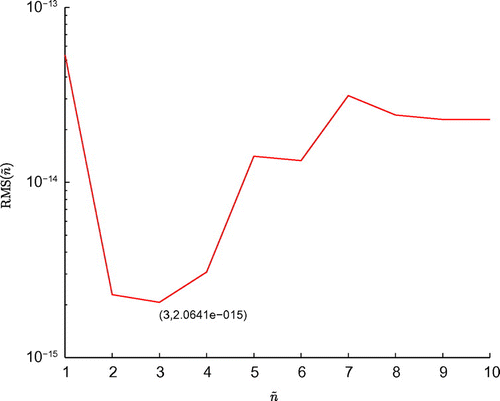
Figure 13. The plots of RMS(c) with respect to c for two classes of initial condition of Example 3 for the rectangular domain: (a) The global initial condition case, (b) The partial initial condition case.

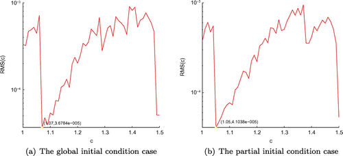
Figure 14. The exact function f(t) and its approximation with four different noise levels added to the measured data, namely $\mathit{\delta }=0.01\%,\mathit{\delta }=0.1\%,\mathit{\delta }=1\%$ and $\mathit{\delta }=5\%$, for the global (Ours) (a) and global (MFS) (b) initial condition cases of Example 3 for the rectangular domain, respectively.

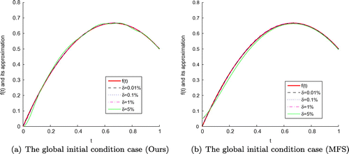
Figure 15. The exact function f(t) and its approximation with four different noise levels added to the measured data, namely $\mathit{\delta }=0.01\%,\mathit{\delta }=0.1\%,\mathit{\delta }=1\%$ and $\mathit{\delta }=5\%$, for the partial (Ours) (a) and partial (MFS) (b) initial condition cases of Example 3 for the rectangular domain, respectively.

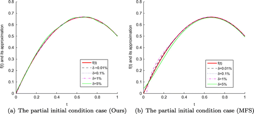
Figure 16. The RMS error (a) of function u(x, y, t) and its maximum error (b) obtained by our proposed scheme with $T=1$, and four different noise levels added to the measured data, namely $\mathit{\delta }=0.01\%,\mathit{\delta }=0.1\%,\mathit{\delta }=1\%$ and $\mathit{\delta }=5\%$, for the global initial condition case of Example 3 for the rectangular domain, L denotes time level corresponding to $t=0,0.1,\dots ,1$.

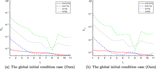
Table 5. The results of $E_{2f}$, $E_{\infty f}$, CPU(s) obtained by our technique and MFS with various error levels, $\mathit{\delta }=0.01\%,\mathit{\delta }=0.1\%,\mathit{\delta }=1\%$ and $\mathit{\delta }=5\%$ for the global initial condition case of Example 3 for the rectangular domain.

		$\mathit{\delta }=0.01\%$	$\mathit{\delta }=0.1\%$	$\mathit{\delta }=1\%$	$\mathit{\delta }=5\%$
	$E_{2f}$	$1.07\times {10}^{-3}$	$1.61\times {10}^{-3}$	$2.46\times {10}^{-3}$	$1.04\times {10}^{-2}$
Ours	$E_{\infty f}$	$3.63\times {10}^{-3}$	$4.64\times {10}^{-3}$	$9.31\times {10}^{-3}$	$3.53\times {10}^{-2}$
	CPU(s)	19.92	19.90	19.99	19.87
	$E_{2f}$	$8.92\times {10}^{-4}$	$1.92\times {10}^{-3}$	$6.71\times {10}^{-3}$	$1.44\times {10}^{-2}$
MFS	$E_{\infty f}$	$2.55\times {10}^{-3}$	$1.03\times {10}^{-2}$	$4.47\times {10}^{-2}$	$4.99\times {10}^{-2}$
	CPU(s)	35.75	35.94	37.00	36.86

Figure 17. The RMS error (a) of function u(x, y, t) and its maximum error (b) obtained by MFS with $T=1$, and four different noise levels added to the measured data, namely $\mathit{\delta }=0.01\%,\mathit{\delta }=0.1\%,\mathit{\delta }=1\%$ and $\mathit{\delta }=5\%$, for the global initial condition case of Example 3 for the rectangular domain, L denotes time level corresponding to $t=0,0.1,\dots ,1$.

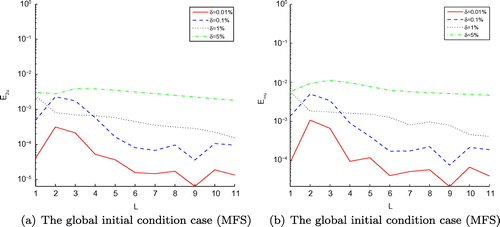
Figure 18. The RMS error (a) of function u(x, y, t) and its maximum error (b) obtained by our method with $T=1$, with four different noise levels added to the measured data, namely $\mathit{\delta }=0.01\%,\mathit{\delta }=0.1\%,\mathit{\delta }=1\%$ and $\mathit{\delta }=5\%$, for the partial initial condition case of Example 3 for the rectangular domain, L denotes time level corresponding to $t=0,0.1,\dots ,1$.

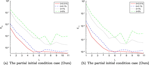
Figure 19. The RMS error (a) of function u(x, y, t) and its maximum error (b) obtained by MFS with $T=1$, with four different noise levels added to the measured data, namely $\mathit{\delta }=0.01\%,\mathit{\delta }=0.1\%,\mathit{\delta }=1\%$ and $\mathit{\delta }=5\%$, for the partial initial condition case of Example 3 for the rectangular domain, L denotes time level corresponding to $t=0,0.1,\dots ,1$.

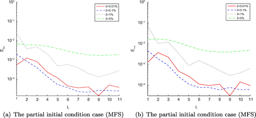
Table 6. The results of $E_{2f}$, $E_{\infty f}$, $E_{2h_2}$, $E_{\infty h_2}$, CPU(s) obtained by our technique and MFS with various error levels, namely $\mathit{\delta }=0.01\%,\mathit{\delta }=0.1\%,\mathit{\delta }=1\%$ and $\mathit{\delta }=5\%$ for the partial initial condition case of Example 3 for the rectangular domain.

		$\mathit{\delta }=0.01\%$	$\mathit{\delta }=0.1\%$	$\mathit{\delta }=1\%$	$\mathit{\delta }=5\%$
	$E_{2f}$	$1.42\times {10}^{-3}$	$1.49\times {10}^{-3}$	$1.58\times {10}^{-3}$	$6.47\times {10}^{-3}$
	$E_{\infty f}$	$2.91\times {10}^{-3}$	$3.18\times {10}^{-3}$	$4.13\times {10}^{-3}$	$1.50\times {10}^{-2}$
Ours	$E_{2h_2}$	$5.06\times {10}^{-3}$	$1.17\times {10}^{-2}$	$1.16\times {10}^{-1}$	$1.95\times {10}^{-1}$
	$E_{\infty h_2}$	$1.50\times {10}^{-2}$	$2.74\times {10}^{-2}$	$3.35\times {10}^{-1}$	$6.29\times {10}^{-1}$
	CPU(s)	20.22	20.15	21.87	21.38
	$E_{2f}$	$4.48\times {10}^{-3}$	$3.41\times {10}^{-3}$	$2.58\times {10}^{-2}$	$1.58\times {10}^{-2}$
	$E_{\infty f}$	$1.32\times {10}^{-2}$	$2.87\times {10}^{-2}$	$1.95\times {10}^{-1}$	$4.39\times {10}^{-2}$
MFS	$E_{2h_2}$	$5.52\times {10}^{-4}$	$2.56\times {10}^{-3}$	$2.70\times {10}^{-2}$	$1.02\times {10}^{-2}$
	$E_{\infty h_2}$	$1.32\times {10}^{-2}$	$5.50\times {10}^{-3}$	$7.75\times {10}^{-2}$	$3.05\times {10}^{-2}$
	CPU(s)	37.21	36.92	36.99	36.86

Figure 20. The error plots between the exact function u(x, y, 0) and its approximation $\tilde{u}(x,y,0)$ obtained by our method with $T=1$, with four different noise levels added to the measured data, namely $\mathit{\delta }=0.01\%,\mathit{\delta }=0.1\%,\mathit{\delta }=1\%$ and $\mathit{\delta }=5\%$ for the partial initial condition case of Example 3 for the rectangular domain.

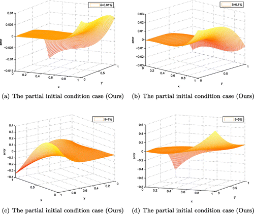
Figure 21. The exact function f(t) and its approximation with four different noise levels added to the measured data, namely $\mathit{\delta }=0.01\%,\mathit{\delta }=0.1\%,\mathit{\delta }=1\%$ and $\mathit{\delta }=5\%$, for the global (Ours) (a) and global (MFS) (b) initial condition cases of Example 3 in the Circular-domain setting, respectively.

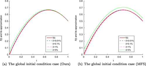
Figure 22. The exact function f(t) and its approximation with four different noise levels added to the measured data, namely $\mathit{\delta }=0.01\%,\mathit{\delta }=0.1\%,\mathit{\delta }=1\%$ and $\mathit{\delta }=5\%$, for the partial (Ours) (a) and partial (MFS) (b) initial condition cases of Example 3 in the Peanut-domain setting, respectively.

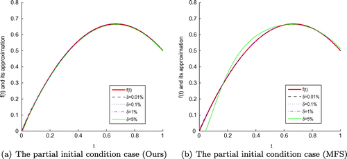
Figure 23. The Circular-domain (a) and the Peanut-domain (b), and the notation "+" denotes the chosen collocation point.

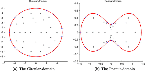
Figure 24. The RMS error (a) of function u(x, y, t) and its maximum error (b) obtained by our proposed scheme with $T=1$, and four different noise levels added to the measured data, namely $\mathit{\delta }=0.01\%,\mathit{\delta }=0.1\%,\mathit{\delta }=1\%$ and $\mathit{\delta }=5\%$, for the global initial condition case of Example 3 in the Circular-domain setting, L denotes time level corresponding to $t=0,0.1,\dots ,1$.

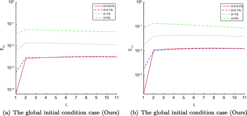
Table 7. The results of $E_{2f}$, $E_{\infty f}$, CPU(s) obtained by our technique and MFS with various error levels, $\mathit{\delta }=0.01\%,\mathit{\delta }=0.1\%,\mathit{\delta }=1\%$ and $\mathit{\delta }=5\%$ for the global initial condition case of Example 3 in the Circular-domain setting.

		$\mathit{\delta }=0.01\%$	$\mathit{\delta }=0.1\%$	$\mathit{\delta }=1\%$	$\mathit{\delta }=5\%$
	$E_{2f}$	$3.18\times {10}^{-3}$	$3.72\times {10}^{-3}$	$5.11\times {10}^{-3}$	$2.33\times {10}^{-2}$
Ours	$E_{\infty f}$	$7.34\times {10}^{-3}$	$2.02\times {10}^{-2}$	$3.61\times {10}^{-2}$	$4.90\times {10}^{-2}$
	CPU(s)	39.84	35.89	34.59	35.45
	$E_{2f}$	$5.56\times {10}^{-3}$	$4.17\times {10}^{-3}$	$1.16\times {10}^{-2}$	$4.41\times {10}^{-2}$
MFS	$E_{\infty f}$	$1.76\times {10}^{-2}$	$1.43\times {10}^{-2}$	$2.24\times {10}^{-2}$	$7.54\times {10}^{-2}$
	CPU(s)	72.63	67.24	67.00	66.63

Figure 25. The RMS error (a) of function u(x, y, t) and its maximum error (b) obtained by MFS with $T=1$, and four different noise levels added to the measured data, namely $\mathit{\delta }=0.01\%,\mathit{\delta }=0.1\%,\mathit{\delta }=1\%$ and $\mathit{\delta }=5\%$, for the global initial condition case of Example 3 in the Circular-domain setting, L denotes time level corresponding to $t=0,0.1,\dots ,1$.

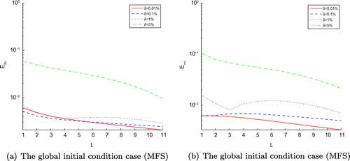
Figure 26. The RMS error (a) of function u(x, y, t) and its maximum error (b) obtained by our method with $T=1$, and four different noise levels added to the measured data, namely $\mathit{\delta }=0.01\%,\mathit{\delta }=0.1\%,\mathit{\delta }=1\%$ and $\mathit{\delta }=5\%$, for the partial initial condition case of Example 3 in the Peanut-domain setting, L denotes time level corresponding to $t=0,0.1,\dots ,1$.

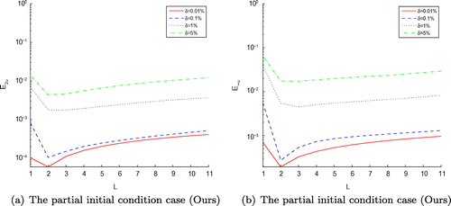
Figure 27. The RMS error (a) of function u(x, y, t) and its maximum error (b) obtained by MFS with $T=1$, and four different noise levels added to the measured data, namely $\mathit{\delta }=0.01\%,\mathit{\delta }=0.1\%,\mathit{\delta }=1\%$ and $\mathit{\delta }=5\%$, for the partial initial condition case of Example 3 in the Peanut-domain setting, L denotes time level corresponding to $t=0,0.1,\dots ,1$.

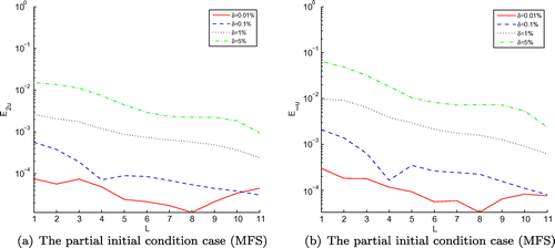
Table 8. The results of $E_{2f}$, $E_{\infty f}$, $E_{2h_2}$, $E_{\infty h_2}$, CPU(s) obtained by our technique and MFS with various error levels, namely $\mathit{\delta }=0.01\%,\mathit{\delta }=0.1\%,\mathit{\delta }=1\%$ and $\mathit{\delta }=5\%$ for the partial initial condition case of Example 3 in the Peanut-domain setting.

		$\mathit{\delta }=0.01\%$	$\mathit{\delta }=0.1\%$	$\mathit{\delta }=1\%$	$\mathit{\delta }=5\%$
	$E_{2f}$	$6.34\times {10}^{-4}$	$1.81\times {10}^{-3}$	$3.81\times {10}^{-3}$	$4.46\times {10}^{-3}$
	$E_{\infty f}$	$1.47\times {10}^{-3}$	$3.55\times {10}^{-3}$	$1.00\times {10}^{-2}$	$1.85\times {10}^{-2}$
Ours	$E_{2h_2}$	$1.08\times {10}^{-4}$	$8.45\times {10}^{-4}$	$7.24\times {10}^{-3}$	$1.61\times {10}^{-2}$
	$E_{\infty h_2}$	$9.65\times {10}^{-4}$	$5.55\times {10}^{-3}$	$3.90\times {10}^{-2}$	$6.48\times {10}^{-2}$
	CPU(s)	36.25	39.72	35.77	35.97
	$E_{2f}$	$2.04\times {10}^{-4}$	$1.39\times {10}^{-3}$	$2.81\times {10}^{-3}$	$3.11\times {10}^{-2}$
	$E_{\infty f}$	$7.11\times {10}^{-4}$	$9.19\times {10}^{-3}$	$1.09\times {10}^{-2}$	$8.83\times {10}^{-2}$
MFS	$E_{2h_2}$	$7.58\times {10}^{-5}$	$5.66\times {10}^{-4}$	$2.62\times {10}^{-3}$	$1.54\times {10}^{-2}$
	$E_{\infty h_2}$	$3.30\times {10}^{-4}$	$2.11\times {10}^{-3}$	$9.70\times {10}^{-3}$	$6.38\times {10}^{-2}$
	CPU(s)	71.59	71.85	71.55	70.73

Xiong XT, Yan YM, Wang JX. A direct numerical method for solving inverse heat source problems. J. Phys.: Conf. Ser. 2011;290:012017

 Google Scholar