Real-time identification of a high-magnitude boundary heat flux on a plate

Figures & data

Figure 1. Geometry of the physical domain.

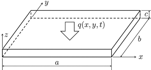
Table 1. Parameters of the heat flux used for case#1.

Quantity	Value (mm)	Quantity	Value (mm)	Quantity	Value
$x_1$	40	$y_1$	40	$q_0$	${10}^7$ W m${}^{-2}$
$x_2$	60	$y_2$	60	$t_0$	0.4 s

Figure 2. Case#1 (a) synthetic measurements and (b) exact heat flux at $t=2.0$ s.

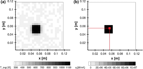
Figure 3. Case#1 estimates at $t=2.0$ s using the classical lumped analysis: (a) temperature and (b) heat flux.

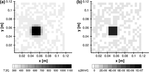
Figure 4. Case#1 time evolution of temperature at z = 0 (a) and heat flux (b) at the selected control volume using the classical lumped analysis.

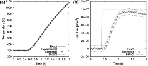
Figure 5. Case#1 analysis of the residuals from classical lumped analysis with heat flux ${10}^7$ W m${}^{-2}$: (a) spatial distribution at $t=2.0$ s and (b) time evolution at the selected control volume.

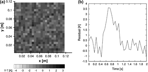
Figure 6. Case#1 estimates at $t=2.0$ s using the improved lumped analysis: (a) temperature and (b) heat flux.

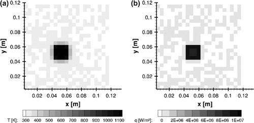
Table 2. Parameters of the heat flux used in the simulation of measurements for Case#2.

Quantity	Value (mm)	Quantity	Value (mm)	Quantity	Value
$x_{1,1}$	30	$y_{1,1}$	30	$q_1$	$5\times {10}^6$ W m${}^{-2}$
$x_{1,2}$	50	$y_{1,2}$	50	$t_1$	0.4 s
$x_{2,1}$	90	$y_{2,1}$	90	$q_2$	${10}^7$ W m${}^{-2}$
$x_{2,2}$	100	$y_{2,2}$	100	$t_2$	0.6 s

Figure 7. Case#1 time evolution of temperature at $z=0$ (a) and heat flux (b) at the selected control volume using the improved lumped analysis.

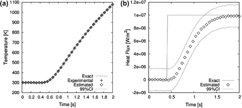
Figure 8. Case#1 analysis of the residuals from improved lumped analysis with unsteady heat flux applied at $z=c$: (a) spatial distribution at $t=2.0$ s and (b) time evolution at the selected control volume.

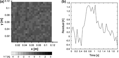
Figure 9. Case#2: (a) synthetic measurements and (b) exact heat flux at $t=2.0$ s.

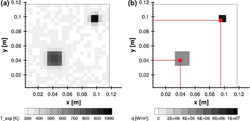
Figure 10. Case#2 estimates at $t=2.0$ s using the classical lumped analysis: (a) temperatures and (b) heat flux.

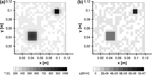
Figure 11. Case#2 time evolution of temperature at $z=0$ (a) and heat flux (b) at the selected control volume at $x=y=40$ mm using the classical lumped analysis.

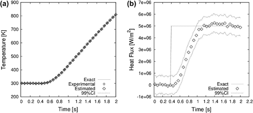
Figure 12. Case#2 time evolution of temperature at $z=0$ (a) and heat flux (b) at the selected control volume at $x=y=95$ mm using the classical lumped analysis.

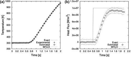
Figure 13. Case#2 time evolution of the residuals from classical lumped analysis: (a) $x=y=40$ mm and (b) $x=y=95$ mm.

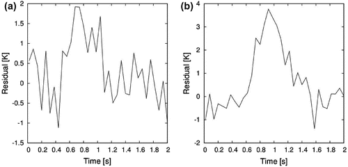
Figure 14. Case#2 spatial distribution of the residuals from classical lumped analysis: (a) $t=0.9$ s and (b) $t=2.0$ s.

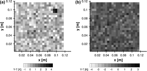
Figure 15. Case#2 estimates at $t=2.0$ s using the improved lumped analysis: (a) temperatures and (b) heat flux.

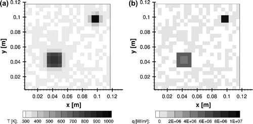
Figure 16. Case#2 time evolution of temperature at $z=0$ (a) and heat flux (b) at the selected control volume at $x=y=40$ mm using the improved lumped analysis.

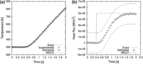
Figure 17. Case#2 time evolution of temperature at $z=0$ (a) and heat flux (b) at the selected control volume at $x=y=95$ mm using the improved lumped analysis.

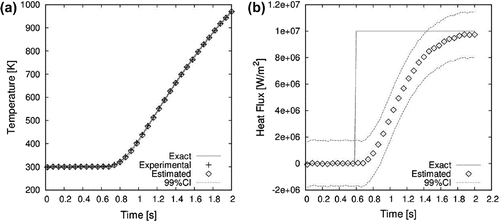
Figure 18. Case#2 time evolution of the residuals from improved lumped analysis: (a) $x=y=40$ mm and (b) $x=y=95$ mm.

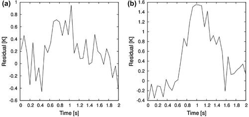
Figure 19. Case#2 spatial distribution of the residuals from classical lumped analysis: (a) $t=0.9$ s and (b) $t=2.0$ s.