Application of artificial bee colony algorithm for inverse modelling of a solar collector

Figures & data

Figure 1. Schematic of double-glazed solar collector.

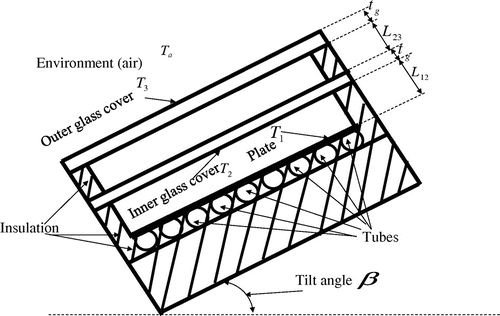
Figure 2. Validation of the forward model; T_a = 303 K (30 °C) and h_a = 25 W/(m² K).

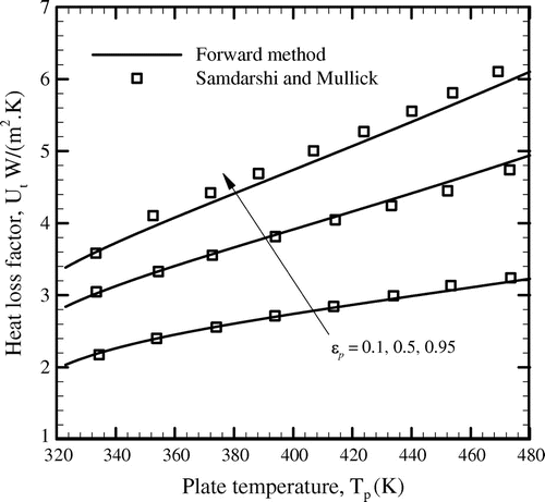
Table 1. Estimated values of parameters for ambient temperature, T_a = 303 K and wind heat transfer coefficient, h_a = 25 W/(m² K).

Forward method	Without measurement error, e = 0 [L12 m, L23 m, ε1, β rad., tg m]	Total size, m
[L12 = L23 = 0.0250 m, ε1 = 0.1000, β = 0.7850 rad., tg = 0.0030 m]	Run 1: [0.0402,0.0256,0.1000,0.1745,0.0036]	0.0730
	Run 2: [0.0377,0.0307,0.1000,0.2436,0.0036]	0.0756
	Run 3: [0.0205,0.0213,0.1129,0.9308,0.0060]	0.0538
	Run 4:[ 0.0358,0.0493,0.1004,0.1746,0.0031]	0.0913
	Run 5: [0.0300, 0.0170,0.1000,0.6968,0.0036]	0.0542
Total size = 0.0560 m	With measurement error, e ≠ 0
	Run 6: [0.0274,0.0500,0.1000,0.3496,0.0060]	0.0894
	Run 7: [0.0182,0.0500,0.1000,0.8478,0.0038]	0.0758
	Run 8: [0.0232,0.0290,0.1000,0.6864, 0.0056]	0.0634
	Run 9: [0.0247,0.0195,0.1000,0.8223,0.0031]	0.0504
	Run 10: [0.0288,0.0500,0.1000,0.5134,0.0033]	0.0854

Figure 3. Comparison of exact and reconstructed heat loss factor distributions; T_a = 303 K (30 °C) and h_a = 25 W/(m² K).

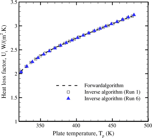
Figure 4. Variation of the objective function with iterations of ABC algorithm (noise-free case); (a) history of 500 iterations, (b) history of first 20 iterations; T_a = 303 K (30 °C) and h_a = 25 W/(m² K).

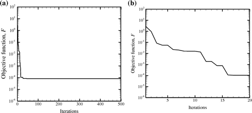
Figure 5. Variation of estimated parameters with iterations of ABC algorithm (noise-free case); T_a = 303 K (30 °C) and h_a = 25 W/(m² K).

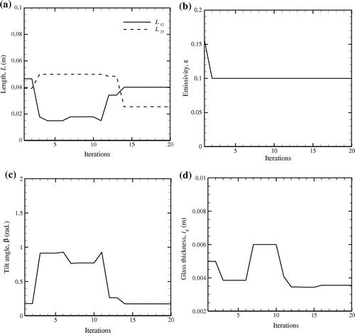
Figure 6. Comparison of exact and reconstructed heat loss factor distributions; $\mathit{\beta }={45}^{\circ }=0.7854\text{rad}.$, L₁₂ = L₂₃ = 0.025 m, t_g = 3 mm, k_g = 1.02 W/(m K), T_a = 303 K (30 °C) and h_a = 25 W/(m² K).

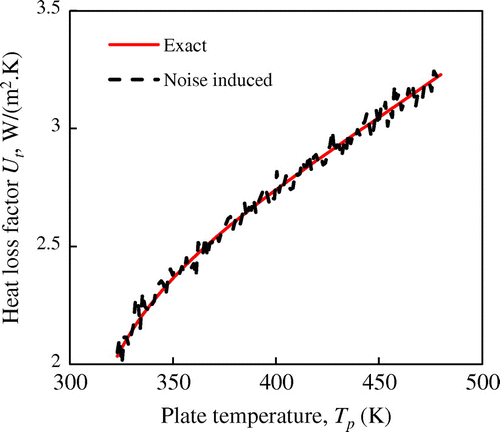
Figure 7. Variation of the objective function with iterations of ABC algorithm (noise-induced case) for Run 6 of Table 1; (a) history of 500 iterations, (b) history of first 20 iterations; T_a = 303 K (30 °C) and h_a = 25 W/(m² K).

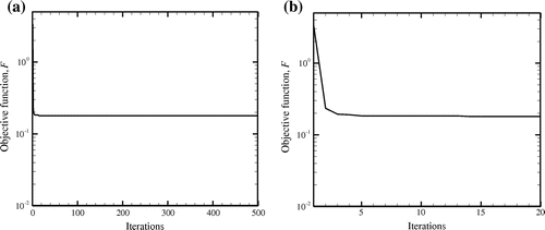
Figure 8. Variation of estimated parameters with iterations of ABC algorithm (noise-induced case) for Run 6 of Table 1; T_a = 303 K (30 °C) and h_a = 25 W/(m² K).

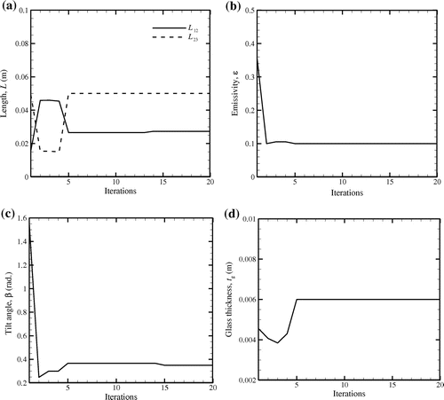
Figure 9. Comparison of sensitivity coefficients of different estimated parameters; $\mathit{\beta }={45}^{\circ }=0.7854\text{rad}$, L₁₂ = L₂₃ = 0.025 m, t_g = 3 mm, k_g = 1.02 W/(m K), T_a = 303 K (30 °C) and h_a = 25 W/(m² K).

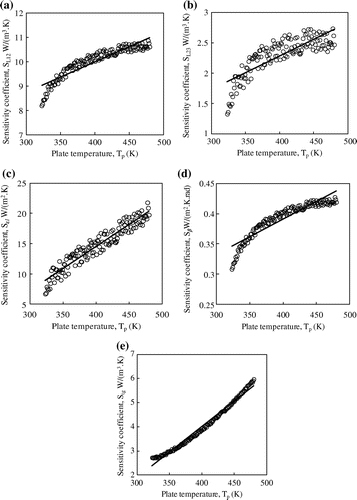
Table 2. Comparison of estimated parameters and objective functions obtained with different optimization methods after 500 iterations.

Forward method	Genetic algorithm	DE algorithm	SA algorithm	ABC algorithm
[L12 = L23 = 0.0250 m, ε1 = 0.1000,  = 0.7850 rad., tg = 0.0030 m]	[L12 = 0.0330 m, L23 = 0.0229 m, ε1 = 0.1007, β = 0.6000 rad., tg = 0.0027 m]	[L12 = 0.0379 m, L23 = 0.0309 m, ε1 = 0.1001, β = 0.2546 rad., tg = 0.0036 m]	[L12 = 0.0249 m, L23 = 0.0269 m, ε1 = 0.1000, β = 0.8250 rad., tg  = 0.0021 m]	[L12 = 0.0209 m, L23 = 0.0200 m, ε1 = 0.1096, β = 0.9061 rad., tg  = 0.0059 m]
	F = 1.800 × 10^−3	F = 1.643 × 10^−3	F = 5.500 × 10^−3	F = 2.939 × 10^−4
Total size 0.0560 m	Total size 0.0613 m	Total size 0.0760 m	Total size 0.0560 m	Total size 0.0527 m

Figure 10. Comparison of objective functions for different optimization algorithms (a) history of 20 iterations, (b) history of 500 iterations; T_a = 303 K (30 °C) and h_a = 25 W/(m² K).

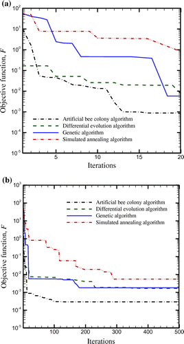
Table 3. Comparison of different optimization methods for 10 additional runs (500 iterations in each case).

Run No.	Genetic algorithm: [L12, L23, ε1, β, tg]; F	DE algorithm: [L12, L23, ε1, β, tg]; F	SA algorithm: [L12, L23, ε1, β, tg]; F	ABC algorithm: [L12, L23, ε1, β, tg]; F
1	[0.0371 m, 0.0355 m, 0.1133, 0.4787 rad., 0.0044 m]; F = 6.300 × 10^−3,(size = 0.0814 m)	[0.0388 m, 0.0299 m, 0.1029, 0.1929 rad., 0.0042 m]; F = 8.805 × 10^−5,(size = 0.0771 m)	[0.0266 m, 0.0204 m, 0.1028, 0.7667 rad., 0.0041 m]; F = 2.938 × 10^−4, (size = 0.0552 m)	[0.0393 m, 0.0267 m, 0.1022, 0.2162 rad., 0.0041 m]; F = 1.569 × 10^−4(size = 0.0742 m)
2	[0.0309 m, 0.0420 m, 0.1067, 0.5626 rad., 0.0039 m]; F = 7.667 × 10^−4, (size = 0.0807 m)	[0.0363 m, 0.0363 m, 0.1000, 0.3155 rad.,0.0030 m]; F = 1.065 × 10^−5, (size = 0.0786 m)	[0.0339 m, 0.0286 m, 0.1008, 0.4956 rad., 0.0031 m]; F = 9.022 × 10^−4, (size = 0.0687 m)	[0.0369 m, 0.0266 m, 0.1048, 0.3764 rad., 0.0047 m];F = 3.210 × 10^−5, (size = 0.0729 m)
3	[0.0234 m, 0.0206 m, 0.1083, 0.8461 rad., 0.0050 m]; F = 6.300 × 10^−3, (size = 0.0540 m)	[0.0269 m, 0.0390 m, 0.1000, 0.7081 rad., 0.0020 m]; F = 5.933 × 10^−4, (size = 0.0699 m)	[0.0434 m, 0.0237 m, 0.1054, 0.2905 rad., 0.0030 m]; F = 8.401 × 10^−3, (size = 0.0731 m)	[0.0346 m, 0.0388 m, 0.1034, 0.3743 rad., 0.0040 m]; F = 3.796 × 10^−4, (size = 0.0814 m)
4	[0.0209 m, 0.0276 m, 0.1027, 0.8751 rad., 0.0039 m]; F = 5.304 × 10^−4, (size = 0.0563 m)	[0.0368 m, 0.0295 m, 0.1039, 0.3671 rad., 0.0040 m]; F = 8.942 × 10^−4, (size = 0.0743 m)	[0.0359 m, 0.0189 m, 0.1078, 0.5503 rad., 0.0050 m]; F = 8.823 × 10^−4, (size = 0.0648 m)	[0.0420 m, 0.0192 m, 0.1069, 0.2594 rad., 0.0053 m]; F = 6.251 × 10^−4, (size = 0.0718 m)
5	[0.0317 m, 0.0455 m, 0.1090, 0.5126 rad., 0.0046 m]; F = 9.667 × 10^−4, (size = 0.0864 m)	[0.0394 m, 0.0309 m, 0.1049, 0.2636 rad., 0.0040 m]; F = 4.129 × 10^−4, (size = 0.0783 m)	[0.0315 m, 0.0401 m, 0.1017, 0.5847 rad., 0.0021 m]; F = 1.276 × 10^−3, (size = 0.0758 m)	[0.0334 m, 0.0333 m, 0.1000, 0.4712 rad., 0.0030 m]; F = 3.165 × 10^−5, (size = 0.0727 m)
6	[0.0245 m, 0.0215 m, 0.1017, 0.7975 rad., 0.0041 m]; F= 1.967 × 10^−4, (size = 0.0542 m)	[0.0338 m, 0.0308 m, 0.1044, 0.4756 rad., 0.0043 m]; F = 6.147 × 10^−5, (size = 0.0732 m)	[0.0375 m, 0.0354 m, 0.1133, 0.4787 rad., 0.0043 m]; F=6.400 × 10^−3, (size = 0.0815 m)	[0.0366 m, 0.0250 m, 0.1027, 0.3922 rad., 0.0043 m]; F = 2.317 × 10^−5, (size = 0.0702 m)
7	[0.0334 m, 0.0204 m, 0.1038, 0.5701 rad., 0.0045 m]; F = 5.234 × 10^−5, (size = 0.0628 m)	[0.0349 m, 0.0260 m, 0.1028, 0.4636 rad., 0.0040 m]; F = 5.831 × 10^−4, (size = 0.0689 m)	[0.0246 m, 0.0280 m, 0.1104, 0.8144 rad., 0.0046 m]; F = 3.900 × 10^−3, (size = 0.0618 m)	[0.0347 m, 0.0346 m, 0.1000, 0.4078 rad., 0.0030 m]; F = 8.997 × 10^−6, (size = 0.0753 m)
8	[0.0393 m, 0.0245 m, 0.1008, 0.2032 rad., 0.0043 m]; F = 6.559 × 10^−4, (size = 0.0724 m)	[0.0150 m, 0.0150 m, 0.1027, 1.0480 rad., 0.0050 m]; F = 3.146 × 10^−3, (size = 0.040 m)	[0.0359 m, 0.0297 m, 0.1014, 0.3908 rad., 0.0036 m]; F = 7.762 × 10^−6, (size = 0.0728 m)	[0.0356 m, 0.0196 m, 0.1049, 0.5064 rad., 0.0049 m]; F= 4.107 × 10^−5, (size = 0.0650 m)
9	[0.0293 m, 0.0440 m, 0.1000, 0.5604 rad., 0.0028 m]; F = 1.684 × 10^−4, (size = 0.0789 m)	[0.0348 m, 0.0347 m, 0.1000, 0.4004 rad., 0.0030 m]; F = 4.951 × 10^−5, (size = 0.0755 m)	[0.0403 m, 0.0216 m, 0.1007, 0.3191 rad., 0.0033 m]; F = 8.907 × 10^−4, (size = 0.0685 m)	[0.0356 m, 0.0352 m, 0.1057, 0.3457 rad., 0.0048 m]; F = 4.148 × 10^−4, (size = 0.0804 m)
10	[0.0319 m, 0.0289 m,0.1138, 0.6112 rad., 0.0059 m]; F = 1.551 × 10^−3, (size = 0.0726 m)	[0.0312 m, 0.0208 m, 0.1019, 0.6227 rad., 0.0041 m]; F = 8.322 × 10^−5, (size = 0.0602 m)	[0.0158 m, 0.0409 m, 0.1056, 0.9904 rad., 0.0040 m]; F = 3.260× 10^−3, (size = 0.0647 m)	[0.0331 m, 0.0331 m,0.1000, 0.4852 rad., 0.0030 m]; F = 1.021 × 10^−5, (size = 0.0722 m)
	Average function, Favg. = 1.748 × 10^−3	Average function, Favg. = 5.922 × 10^−4	Average function, Favg. = 2.621 × 10^−3	Average function, Favg. = 1.723 × 10^−4

Table 4. Estimated values of parameters for variable ambient conditions.

Forward method	[L12 m, L23 m, ε1, β rad., tg m]	Total size, m
[L12 = L23 = 0.0250 m, ε1 = 0.1000, β = 0.7850 rad., tg = 0.0030 m] Total size = 0.0560 m	Ta = 295 K (22 °C), ha = 20 W/(m^2.K) Run 1: [0.0150,0.0150,0.1000,1.0617,0.0039]	0.0378
	Ta = 308 K (35 °C), ha = 30 W/(m^2.K) Run 2: [0.0333,0.0498,0.1000,0.4569,0.0017]	0.0865
	Ta = 290 K (17 °C), ha = 28 W/(m^2.K) Run 3: [0.0272,0.0171,0.1000,0.7657,0.0037]	0.0517

Figure 11. Comparison of objective functions for solar collector operating under varying ambient conditions (a) history of 200 iterations, (b) history of first 20 iterations.

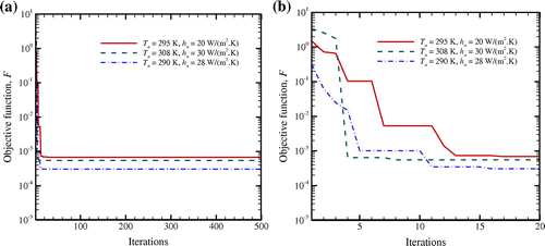
Figure 12. Variation of estimated parameters for ambient temperature, T_a = 295 K (22 °C) and wind heat transfer coefficient, h_a = 20 W/(m² K).

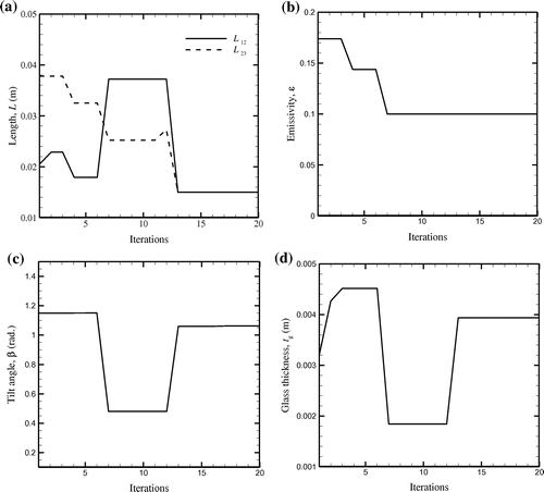
Figure 13. Variation of estimated parameters for ambient temperature, T_a = 308 K (35 °C) and wind heat transfer coefficient, h_a = 30 W/(m² K).

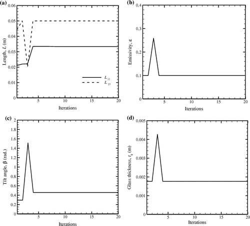
Figure 14. Variation of estimated parameters for ambient temperature, T_a = 290 K (17 °C) and wind heat transfer coefficient, h_a = 28 W/(m² K).

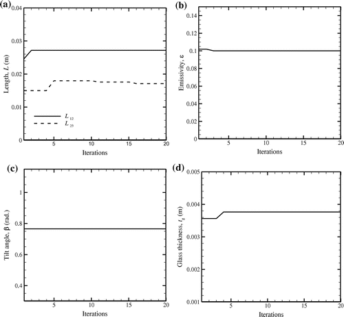
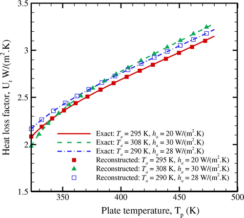
Figure 15. Comparison of exact and reconstructed heat loss factor distributions under different environmental conditions.