610
Views
16
CrossRef citations to date
0
Altmetric
Articles

An adjoint method in inverse problems of chromatography

ORCID Icon, , , , &
Pages 1112-1137 | Received 14 Mar 2016, Accepted 04 Aug 2016, Published online: 24 Aug 2016

Figures & data

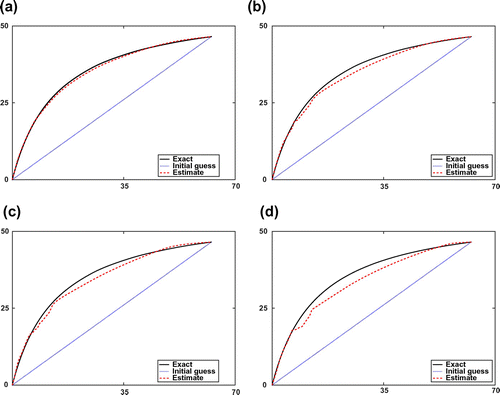
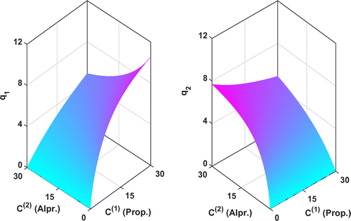
Figure 1. Estimated adsorption isotherms by synthetic data with different error levels δ of and their corresponding relative errors Δ. (a) δ=0 and Δ=0.0154. (b) δ=1% and Δ=0.0404. (c) δ=5% and Δ=0.0520. (d) δ=10% and Δ=0.0790.

Figure 1. Estimated adsorption isotherms by synthetic data with different error levels δ of and their corresponding relative errors Δ. (a) δ=0 and Δ=0.0154. (b) δ=1% and Δ=0.0404. (c) δ=5% and Δ=0.0520. (d) δ=10% and Δ=0.0790.

Table 1. Estimated adsorption isotherms and computational costs (the number objective function evaluation (NOFE)) of the boundary fitting method (BF) and the Kohn–Vogelius method (KV) with different error levels for both the Equilibrium-Dispersive (ED) model and the Transport-Dispersive (TD) model with the given mass transfer resistance kf=[95,135]T.

Table 2. Estimated adsorption isotherm parameters and mass transfer resistance by the boundary fitting method (BF) and the Kohn–Vogelius method (KV) with different error levels in the Transport-Dispersive (TD) model.

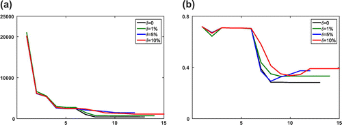
Figure 2. Numerical results of the boundary fitting method for the Equilibrium-Dispersive model with different error levels δ at every iteration step l. (a) The value of objective function JBF,α and (b) the relative error ξl-ξ¯2/ξl2 of recovered parameters.

Figure 2. Numerical results of the boundary fitting method for the Equilibrium-Dispersive model with different error levels δ at every iteration step l. (a) The value of objective function JBF,α and (b) the relative error ‖ξl-ξ¯‖2/‖ξl‖2 of recovered parameters.

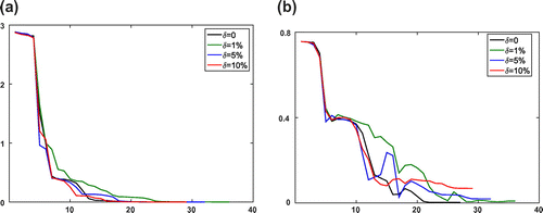
Figure 3. Numerical results of KV method for the Equilibrium-Dispersive model with different error levels δ at every iteration step l. (a) The value of objective function JKV,α and (b) the relative error ξl-ξ¯2/ξl2 of recovered parameters.

Figure 3. Numerical results of KV method for the Equilibrium-Dispersive model with different error levels δ at every iteration step l. (a) The value of objective function JKV,α and (b) the relative error ‖ξl-ξ¯‖2/‖ξl‖2 of recovered parameters.

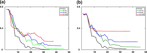
Figure 4. The relative error of estimated adsorption isotherm parameters for the Transport-Dispersive model with different error levels δ at every iteration step l. (a) The boundary fitting method and (b) the Kohn–Vogelius method.
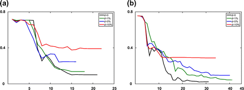
Figure 4. The relative error of estimated adsorption isotherm parameters for the Transport-Dispersive model with different error levels δ at every iteration step l. (a) The boundary fitting method and (b) the Kohn–Vogelius method.

Figure 5. The relative errors of estimated adsorption isotherms and mass transfer resistance for the Transport-Dispersive model with different error levels δ at every iteration step l. (a) The relative errors of estimated adsorption isotherms ξl-ξ¯2/ξl2 and (b) The relative errors of estimated mass transfer kfl-kf2/kfl2.

Figure 5. The relative errors of estimated adsorption isotherms and mass transfer resistance for the Transport-Dispersive model with different error levels δ at every iteration step l. (a) The relative errors of estimated adsorption isotherms ‖ξl-ξ¯‖2/‖ξl‖2 and (b) The relative errors of estimated mass transfer ‖kfl-kf‖2/‖kfl‖2.

Figure 6. The reconstructed adsorption isotherms by KV method for the Equilibrium-Dispersive model.

Figure 6. The reconstructed adsorption isotherms by KV method for the Equilibrium-Dispersive model.

Figure 7. The reconstructed adsorption isotherms by KV method for the Transport-Dispersive model. (a) Fixed mass transfer resistance kf(1)=95 and kf(2)=195. (b) Estimating mass transfer resistance by inverse algorithm with the constraints 20kf(i)400, i=1,2.

Figure 7. The reconstructed adsorption isotherms by KV method for the Transport-Dispersive model. (a) Fixed mass transfer resistance kf(1)=95 and kf(2)=195. (b) Estimating mass transfer resistance by inverse algorithm with the constraints 20≤kf(i)≤400, i=1,2.

Figure 8. A comparison between the experimental elution profile (solid line) and the simulated total elution profile (dashed line) corresponds to the estimated parameter ξ^ in the Equilibrium-Dispersive model. (a) Injection profile h(t)=[0.75,0]mM. (b) Injection profile h(t)=[0,15]mM.

Figure 8. A comparison between the experimental elution profile (solid line) and the simulated total elution profile (dashed line) corresponds to the estimated parameter ξ^ in the Equilibrium-Dispersive model. (a) Injection profile h(t)=[0.75,0]mM. (b) Injection profile h(t)=[0,15]mM.

Figure 9. (a) A comparison between the experimental elution profile (solid line) with injection h(t)=[0.75,0.75]mM and the simulated total elution profile (dashed line) corresponds to the estimated parameter ξ^. (b) The value of objective function JBV,α in the logarithmic scale at every iteration step l.

Figure 9. (a) A comparison between the experimental elution profile (solid line) with injection h(t)=[0.75,0.75]mM and the simulated total elution profile (dashed line) corresponds to the estimated parameter ξ^. (b) The value of objective function JBV,α in the logarithmic scale at every iteration step l.

Reprints and Corporate Permissions

Please note: Selecting permissions does not provide access to the full text of the article, please see our help page How do I view content?

To request a reprint or corporate permissions for this article, please click on the relevant link below:

Academic Permissions

Please note: Selecting permissions does not provide access to the full text of the article, please see our help page How do I view content?

Obtain permissions instantly via Rightslink by clicking on the button below:

If you are unable to obtain permissions via Rightslink, please complete and submit this Permissions form. For more information, please visit our Permissions help page.