
Figures & data
Figure 1. Local support domains for an arbitrary nodal point for two-dimensional hypothesis domain.
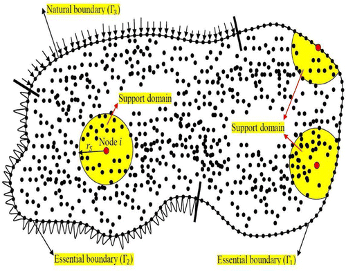
Figure 2. Considered domains in the current paper.
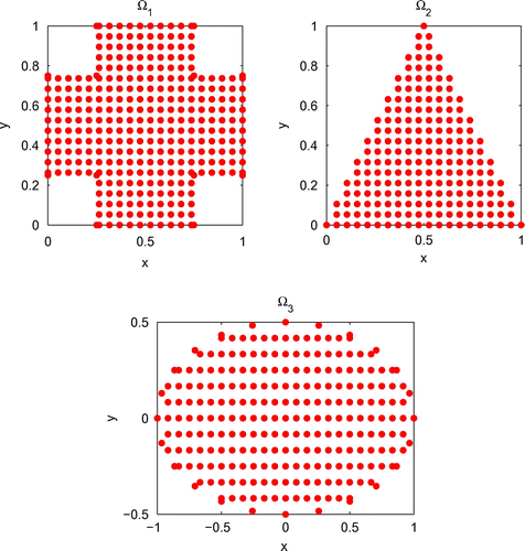
Figure 3. and
profiles for different noise levels with
,
and
on
for Example 1.
![Figure 3. uapprox and ε∞(u) profiles for different noise levels with N=625, δt=0.01 and T=1 on [0,1]2 for Example 1.](/cms/asset/071399fd-dea5-431e-aec1-9d6d0c423e02/gipe_a_1289194_f0003_oc.gif)
Figure 4. The exact solutions in comparison with the regularized numerical solutions for
,
,
and
on
for Example 1.
![Figure 4. The exact solutions {r(t),u(x,0.5,T)} in comparison with the regularized numerical solutions for N=625, δt=0.01, σ∈{1,2,3}% and T=1 on [0,1]2 for Example 1.](/cms/asset/7e3a3a5d-e440-4dfe-9ad0-76f2be987dc5/gipe_a_1289194_f0004_oc.gif)
Figure 5. Condition number and regularization parameter values for with
,
and
on
for Example 1.
![Figure 5. Condition number and regularization parameter values for k=1:T/δt¯ with N=121, δt=0.01 and T=1 on [0,1]2 for Example 1.](/cms/asset/9dad8592-aae8-4513-a311-a96197bcd178/gipe_a_1289194_f0005_oc.gif)
Figure 6. Graphs of approximate solution and absolute error of (a) and (b) with approximate solution and absolute error of r(t) (c) and (d) in the case of no regularization and
,
and
on domain
for Example 1.
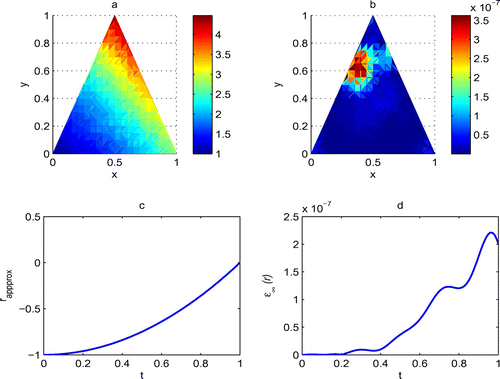
Figure 7. (left) and
(right) profiles for different noise levels with
,
and
on
for Example 2.
![Figure 7. uapprox (left) and ε∞(u) (right) profiles for different noise levels with N=625, δt=0.01 and T=1 on [0,1]2 for Example 2.](/cms/asset/3e7b979c-85f8-42cb-8df5-59d6fe695cc7/gipe_a_1289194_f0007_oc.gif)
Table 1. Numerical results of absolute errors and relative errors on with
,
,
and condition number
for Example 1.
Table 2. Numerical results of absolute errors, relative errors and condition numbers on with
and
for Example 1.
Figure 8. Graphs of absolute errors r(t) and u(x, y, T) using the SMRPI with ,
,
and
on
for Example 2.
![Figure 8. Graphs of absolute errors r(t) and u(x, y, T) using the SMRPI with σ∈{0,3,5}%, N∈{121,225,441,625,1089,1849,2209}, δt=0.02 and T=1 on [0,1]2 for Example 2.](/cms/asset/aa3258b7-3421-4b86-bd8b-8e168adfbc36/gipe_a_1289194_f0008_oc.gif)
Figure 9. Condition number and regularization parameter values for with
,
and
on
for Example 2.
![Figure 9. Condition number and regularization parameter values for k=1:T/δt¯ with N=2209, δt=0.02 and T=1 on [0,1]2 for Example 2.](/cms/asset/21ea6ac8-760b-4e18-b7cf-e681636f3aa0/gipe_a_1289194_f0009_oc.gif)
Figure 10. Graphs of approximate solution and absolute error of (a,b) with approximate solution and absolute error of r(t) (c,d) in the case of no regularization and
,
and
on domain
for Example 2.
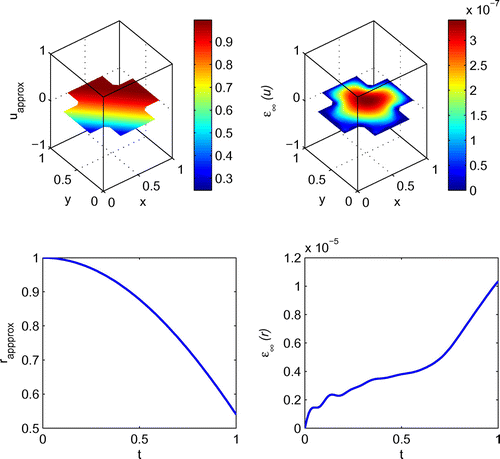
Table 3. Numerical results of absolute errors and relative errors on with
,
,
and condition number
for Example 2.
Figure 11. (left) and
(right) profiles for different noise levels with
,
and
on
for Example 3.
![Figure 11. uapprox (left) and ε∞(u) (right) profiles for different noise levels with N=625, δt=0.01 and T=1 on [0,1]2 for Example 3.](/cms/asset/5fd72930-bdd7-48f4-99e8-82cef3704ed8/gipe_a_1289194_f0011_oc.gif)
Figure 12. Graphs of relative errors r(t) and u(x, y, T) using the SMRPI with ,
,
and
on
for Example 3.
![Figure 12. Graphs of relative errors r(t) and u(x, y, T) using the SMRPI with σ∈{0,3,5}%, N∈{121,225,441,625,1089,1681}, δt=0.02 and T=1 on [0,1]2 for Example 3.](/cms/asset/2fe80203-853e-4806-9e70-dc74603d0a37/gipe_a_1289194_f0012_oc.gif)
Figure 13. Condition number and regularization parameter values for with
,
and
on
for Example 3.
![Figure 13. Condition number and regularization parameter values for k=1:T/δt¯ with N=441, δt=0.02 and T=1 on [0,1]2 for Example 3.](/cms/asset/b682b442-0020-4e6d-8266-09922dda0774/gipe_a_1289194_f0013_oc.gif)
Figure 14. Graphs of approximate solution and absolute error of (a,b) with approximate solution and absolute error of r(t) (c,d) in the case of no regularization and
,
and
on domain
for Example 3.
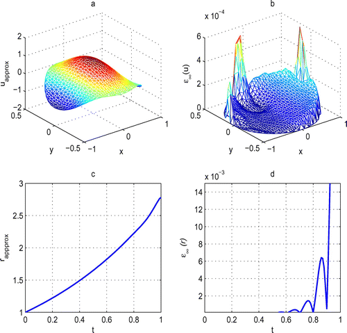
Table 4. Numerical results of absolute errors with no regularization and , on irregular domains
,
and
for Example 2.
Table 5. Numerical results of absolute errors and relative errors on with
,
,
and condition number
for Example 3.