465
Views
1
CrossRef citations to date
0
Altmetric
Articles

Multi-model method for solving nonlinear transient inverse heat conduction problems

ORCID Icon, , &
Pages 621-640 | Received 26 Dec 2015, Accepted 09 May 2017, Published online: 12 Jun 2017

Figures & data

Figure 1. (a) One-dimensional transient heat conduction system. (b) Grid division of time and space.
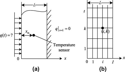
Figure 1. (a) One-dimensional transient heat conduction system. (b) Grid division of time and space.

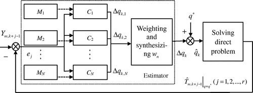
Figure 2. Block scheme of the multi-model inversion system.

Figure 2. Block scheme of the multi-model inversion system.

Table 1. Thermal properties of Armco (99.75% pure) [Citation20].

Figure 3. Comparison of temperature evolution calculated by the heat balance method in this work and the finite element software Comsol.
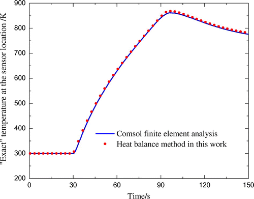
Figure 3. Comparison of temperature evolution calculated by the heat balance method in this work and the finite element software Comsol.

Table 2. Effect of the number of local models on the inversion results.

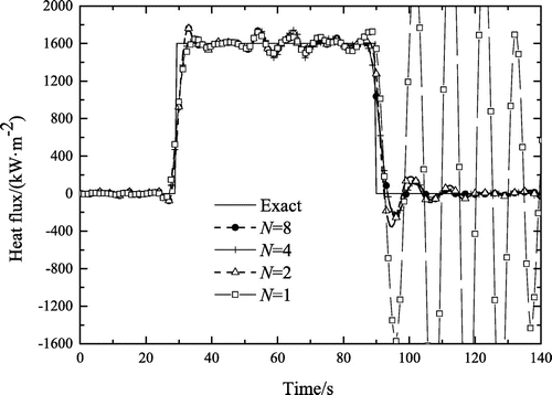
Figure 4. Inversion results of the multi-model method with different numbers of local models.

Figure 4. Inversion results of the multi-model method with different numbers of local models.

Table 3. Comparison of the single model, adaptive model and multi-model method.

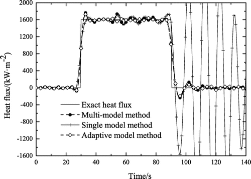
Figure 5. Comparison of the single model, adaptive model and multi-model method.

Figure 5. Comparison of the single model, adaptive model and multi-model method.

Figure 6. DMC digital filter coefficients at different balance point temperatures (α=1×10⁻¹⁰ K2 m4 W−2, kp = 30, kf = 10, tk = 18 s).
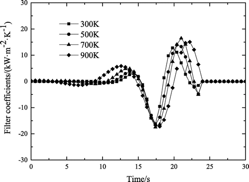
Figure 6. DMC digital filter coefficients at different balance point temperatures (α=1×10⁻¹⁰ K2 m4 W−2, kp = 30, kf = 10, tk = 18 s).

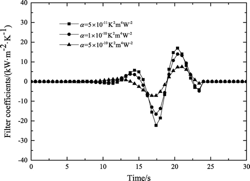
Figure 7. The DMC digital filter coefficients for α = 5 × 10−10, 1 × 10−10 and 5 × 10−11 K2 m4 W−2 (kp = 30, kf = 10, tk = 18 s, vb,n = 600 K).

Figure 7. The DMC digital filter coefficients for α = 5 × 10−10, 1 × 10−10 and 5 × 10−11 K2 m4 W−2 (kp = 30, kf = 10, tk = 18 s, vb,n = 600 K).

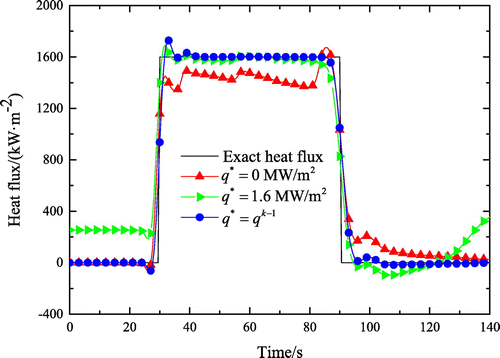
Figure 8. Effect of the initial guess value of the surface heat flux on the inversion results by DMC filter. (α=1×10⁻¹⁰ K2 m4 W−2)

Figure 8. Effect of the initial guess value of the surface heat flux on the inversion results by DMC filter. (α=1×10⁻¹⁰ K2 m4 W−2)

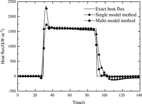
Figure 9. Comparison of the inversion results of multi-model and single model method associated with DMC digital filter with noisy-free measured temperature. (α=1×10⁻¹⁰ K2 m4 W−2, kp = 20, kf = r = 10).

Figure 9. Comparison of the inversion results of multi-model and single model method associated with DMC digital filter with noisy-free measured temperature. (α=1×10⁻¹⁰ K2 m4 W−2, kp = 20, kf = r = 10).

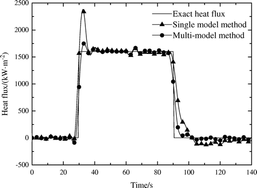
Figure 10. Comparison of the inversion results of multi-model and single model method associated with DMC digital filter with σ=0.5 K. (α=1×10⁻¹⁰ K2 m4 W−2, kp = 20, kf = r = 10).

Figure 10. Comparison of the inversion results of multi-model and single model method associated with DMC digital filter with σ=0.5 K. (α=1×10⁻¹⁰ K2 m4 W−2, kp = 20, kf = r = 10).

Reprints and Corporate Permissions

Please note: Selecting permissions does not provide access to the full text of the article, please see our help page How do I view content?

To request a reprint or corporate permissions for this article, please click on the relevant link below:

Academic Permissions

Please note: Selecting permissions does not provide access to the full text of the article, please see our help page How do I view content?

Obtain permissions instantly via Rightslink by clicking on the button below:

If you are unable to obtain permissions via Rightslink, please complete and submit this Permissions form. For more information, please visit our Permissions help page.