480
Views
5
CrossRef citations to date
0
Altmetric
Original Articles

The method of fundamental solution for the inverse source problem for the space-fractional diffusion equation

ORCID Icon &
Pages 925-941 | Received 10 Jan 2017, Accepted 15 Aug 2017, Published online: 04 Sep 2017

Figures & data

Figure 1. The analytical f(t) and its approximation f(t) when there is no regularization method for Example 1.
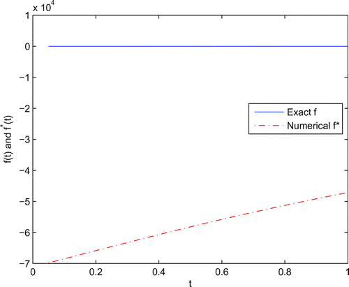
Figure 1. The analytical f(t) and its approximation f∗(t) when there is no regularization method for Example 1.

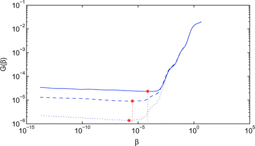
Figure 2. The GCV function obtained for various levels of noise added into the measured data, namely δ=1%(....), δ=3%(--) and δ=5%(-), with n=m=s=20, T=2.5, X=-1 for Example 1.

Figure 2. The GCV function obtained for various levels of noise added into the measured data, namely δ=1%(....), δ=3%(--) and δ=5%(-), with n=m=s=20, T=2.5, X=-1 for Example 1.

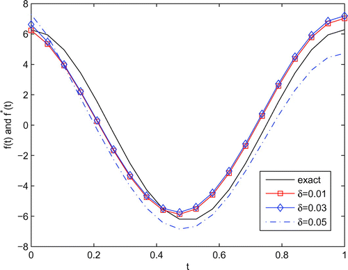
Figure 3. The analytical f(t) and its approximation f(t) with n=m=s=20, T=2.5, X=-1, and various levels of noise added into the measured data, namely δ=1%, δ=3% and δ=5% for Example 1.

Figure 3. The analytical f(t) and its approximation f∗(t) with n=m=s=20, T=2.5, X=-1, and various levels of noise added into the measured data, namely δ=1%, δ=3% and δ=5% for Example 1.

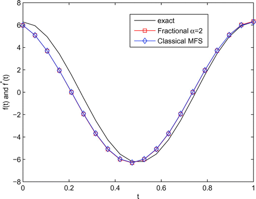
Figure 4. The analytical f(t) and its approximation f(t) with n=m=s=20, T=2.5, X=-1 for fractional MFS (α=2) and n=m=s=20, T=2.5 for classical MFS when level of noise added into the measured data δ=1% for Example 1.

Figure 4. The analytical f(t) and its approximation f∗(t) with n=m=s=20, T=2.5, X=-1 for fractional MFS (α=2) and n=m=s=20, T=2.5 for classical MFS when level of noise added into the measured data δ=1% for Example 1.

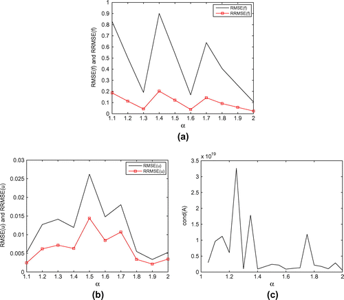
Figure 5. (a) The RMSE(f) and RRMSE(f) of the numerical solutions for Example 1 with n=m=s=20, δ=1%, T=2.5, X=-1 and x0=0.5 with respect to the fractional order α; (b) The RMSE(u) and RRMSE(u) of the numerical solutions for Example 1 with n=m=s=20, δ=1%, T=2.5, X=-1 and x0=0.5 with respect to the fractional order α; (c) The condition number cond(A) of A with n=m=s=20, T=2.5, X=-1 and x0=0.5 with respect to the fractional order α.

Figure 5. (a) The RMSE(f) and RRMSE(f) of the numerical solutions for Example 1 with n=m=s=20, δ=1%, T=2.5, X=-1 and x0=0.5 with respect to the fractional order α; (b) The RMSE(u) and RRMSE(u) of the numerical solutions for Example 1 with n=m=s=20, δ=1%, T=2.5, X=-1 and x0=0.5 with respect to the fractional order α; (c) The condition number cond(A) of A with n=m=s=20, T=2.5, X=-1 and x0=0.5 with respect to the fractional order α.

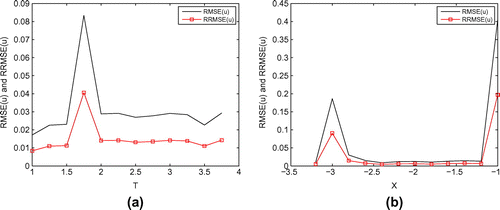
Figure 6. (a) The RMSE(u) and RRMSE(u) of the numerical solutions for Example 1 with δ=1%, x0=0.2, X=-1 with respect to the parameter T; (b) The RMSE(u) and RRMSE(u) of the numerical solutions for Example 1 with δ=1%, x0=0.5, T=2.5 with respect to the parameter X.

Figure 6. (a) The RMSE(u) and RRMSE(u) of the numerical solutions for Example 1 with δ=1%, x0=0.2, X=-1 with respect to the parameter T; (b) The RMSE(u) and RRMSE(u) of the numerical solutions for Example 1 with δ=1%, x0=0.5, T=2.5 with respect to the parameter X.

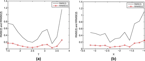
Figure 7. (a) The RMSE(f) and RRMSE(f) of the numerical solutions for Example 1 with δ=1%, x0=0.5, X=-1 with respect to the parameter T; (b) The RMSE(f) and RRMSE(f) of the numerical solutions for Example 1 with δ=1%, x0=0.5, T=2.5 with respect to the parameter X.

Figure 7. (a) The RMSE(f) and RRMSE(f) of the numerical solutions for Example 1 with δ=1%, x0=0.5, X=-1 with respect to the parameter T; (b) The RMSE(f) and RRMSE(f) of the numerical solutions for Example 1 with δ=1%, x0=0.5, T=2.5 with respect to the parameter X.

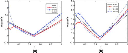
Figure 8. (a) The analytical f(t) and its approximation f(t) with n=m=s=25, T=1.5, X=-1, and various levels of noise added into the measured data, namely δ=1%, δ=3% and δ=5%  for  Example 2; (b) The analytical f(t) and its approximation f(t) with n=m=s=30, T=2, X=-1, and various levels of noise added into the measured data,namely δ=1%, δ=3% and δ=5% for Example 2.

Figure 8. (a) The analytical f(t) and its approximation f∗(t) with n=m=s=25, T=1.5, X=-1, and various levels of noise added into the measured data, namely δ=1%, δ=3% and δ=5%  for  Example 2; (b) The analytical f(t) and its approximation f∗(t) with n=m=s=30, T=2, X=-1, and various levels of noise added into the measured data,namely δ=1%, δ=3% and δ=5% for Example 2.

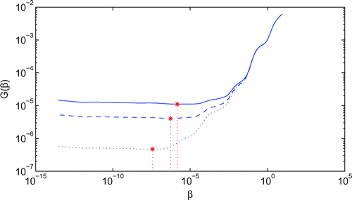
Figure 9. The GCV function obtained for various levels of noise added into the measured data, namely δ=1%(....), δ=3%(--) and δ=5%(-), with n=m=s=25, T=2.5, X=-1 for Example 2.

Figure 9. The GCV function obtained for various levels of noise added into the measured data, namely δ=1%(....), δ=3%(--) and δ=5%(-), with n=m=s=25, T=2.5, X=-1 for Example 2.

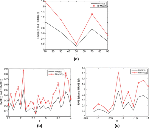
Figure 10. (a) The accuracy of the numerical solutions for Example 2 with δ=1%,x0=0.9,X=-1 and T=2.5 with respect to the parameter n; (b) The accuracy of the numerical solutions for Example 2 with δ=1%, x0=0.9, X=-1 with respect to the parameter T; (c) The accuracy of the numerical solutions for Example 2 with δ=1%, x0=0.9, T=1.5 with respect to the parameter X.

Figure 10. (a) The accuracy of the numerical solutions for Example 2 with δ=1%,x0=0.9,X=-1 and T=2.5 with respect to the parameter n; (b) The accuracy of the numerical solutions for Example 2 with δ=1%, x0=0.9, X=-1 with respect to the parameter T; (c) The accuracy of the numerical solutions for Example 2 with δ=1%, x0=0.9, T=1.5 with respect to the parameter X.

Table 1. The values of cond(A), RMSE(u), RRMSE(u), RMSE(f), RRMSE(f) for various values of X in Example 1, δ=1%, T=2.5.

Table 2. The values of cond(A), RMSE(u), RRMSE(u), RMSE(f), RRMSE(f) for various values of T in Example 1, δ=1%, X=-1.

Table 3. The values of RRMSE(f) for various values of δ and x0 in Example 1, T=2.5, X=-1.

Reprints and Corporate Permissions

Please note: Selecting permissions does not provide access to the full text of the article, please see our help page How do I view content?

To request a reprint or corporate permissions for this article, please click on the relevant link below:

Academic Permissions

Please note: Selecting permissions does not provide access to the full text of the article, please see our help page How do I view content?

Obtain permissions instantly via Rightslink by clicking on the button below:

If you are unable to obtain permissions via Rightslink, please complete and submit this Permissions form. For more information, please visit our Permissions help page.