An efficient method to estimate sorption isotherm curve coefficients

Figures & data

Figure 1. Illustration of the discrepancies observed when comparing experimental data to results from numerical models of moisture transfer in porous material.

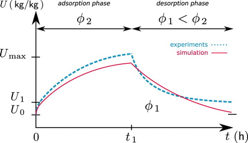
Figure 2. Illustration of the RH-box experimental facility.

Figure 3. Sensors of relative humidity and temperature (a) and wood fibre samples (b) with white acrylic seal and with aluminium tape.

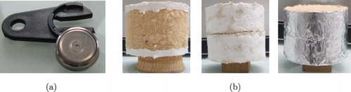
Table 1. A priori dimensionless material properties of wood fibre from [23,33].

Storage coefficient c	$c\left(u\right)=c_0+c_{1}u+c_2{u}^2$
	$c_0=1$, $c_1=-9.79\cdot {10}^{-1}$, $c_2=1.06$
Diffusion coefficient d	$d\left(u\right)=d_0+d_{1}u$
	$d_0=1$, $d_1=0.29$
PÉCLET number	$\text{P'e}=1.1\cdot {10}^{-2}$
FOURIER number	$\text{Fo}=4\cdot {10}^{-3}$
BIOT number	$\text{Bi}=13.7$

Table 2. Possible designs according to the experimental facility.

			Multiple step
Single step			Case 1				Case 2
Design	$u_{\mathrm{i}}$	$u_{\mathrm{c}}$	Design	τ	Design	τ	Design	τ	Design	τ
1	0.2	0.66	5	1	9	5	13	1	17	5
2	0.2	1.5	6	2	10	6	14	2	18	6
3	0.66	1.5	7	3	11	7	15	3	19	7
4	1.5	0.66	8	4	12	8	16	4	20	8

Case 1: $u_{\mathrm{i}}=0.2$, $u_{\mathrm{c}}^1=0.66$, $u_{\mathrm{c}}^2=1.5$, $u_{\mathrm{c}}^3=0.66$.

Case 2: $u_{\mathrm{i}}=0.2$, $u_{\mathrm{c}}^1=1.5$, $u_{\mathrm{c}}^2=0.66$, $u_{\mathrm{c}}^3=1.5$.

Figure 4. Variation of the criterion Ψ for the four possible single-step designs (a) and as a function of the sensor position X for the OED (b), in the case of estimating one parameter.

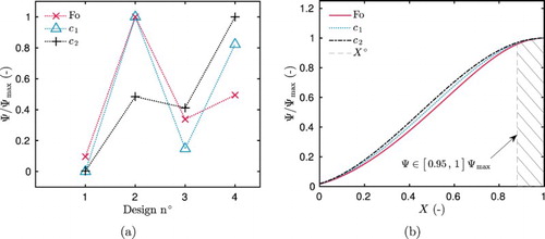
Figure 5. Sensitivity coefficients Θ for parameters $\text{Fo}$, $c_1$ and $c_2$ for the OED (a) and for design 1 (b) ($X=X^{\circ }$).

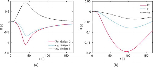
Figure 6. Variation of the criterion Ψ for the 16 possible designs (a) and as a function of the sensor position X for the OED (b), in the case of estimating one parameter.

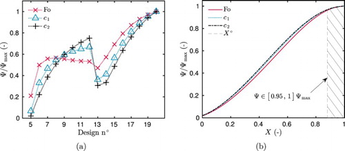
Figure 7. Sensitivity coefficients Θ for parameters $\text{Fo}$, $c_1$ and $c_2$ for the OED (design 20) (a), design 12 (b), design 5 (c) and design 13 (d) ($X=X^{\circ }$).

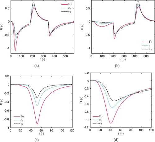
Figure 8. Variation of the criterion Ψ for the four possible designs of single step of relative humidity (a) and as a function of the sensor position X for the OED (b), in the case of estimating the couple of parameters $(\text{Fo},c_2)$.

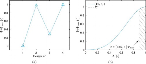
Figure 9. Variation of the criterion Ψ for the 16 possible designs of multiple steps of relative humidity (a) and as a function of the sensor position X for the OED (b), in the case of estimating the couple of parameters $(\text{Fo},c_2)$.

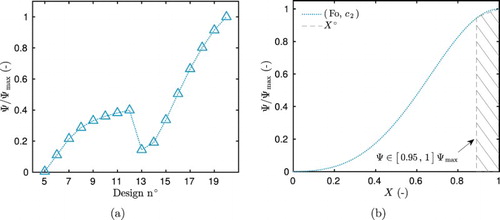
Table 3. Synthesis of the tests carried out with the expression of the cost function.

	Tests
Definition of the cost function $\text{J}$	1	2	3	4	5	6	7	8	9
Experiments considered separately	x	x	x
Experiments at the same time (3 parameters to estimate)				x	x	x
Experiments at the same time (5 parameters to estimate)							x	x	x
Euclidean norm	x			x			x
Infinite norm		x			x			x
Sum of the infinite norms			x			x			x

Figure 10. Residual between the measured data and numerical results for both experiments (a) and number of computations of the direct problem (b) for the different definition of the cost function $\text{J}$.

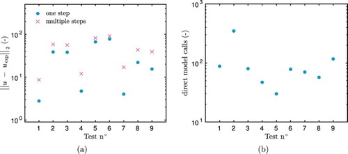
Figure 11. Comparison of the numerical results with the experimental data (a–b) and their $98\mathrm{\%}$ confidence interval for the single-step (a) and the multiple-step (b) experiments (test 1). Comparison of the residual for the single-step (c) and multiple-step (d) experiments.

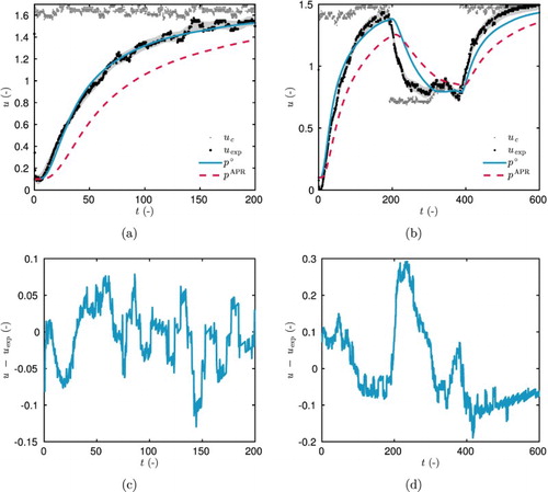
Figure 12. Convergence of the parameter estimation, for the test 1 as a function of the number of iterations (a) and number of computations of the direct model (b).

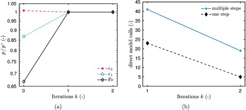
Figure 13. Probability density function approximated for the estimated parameters, computed using the sensitivity of single-step (c) and a multiple-step (a–b) experiments.

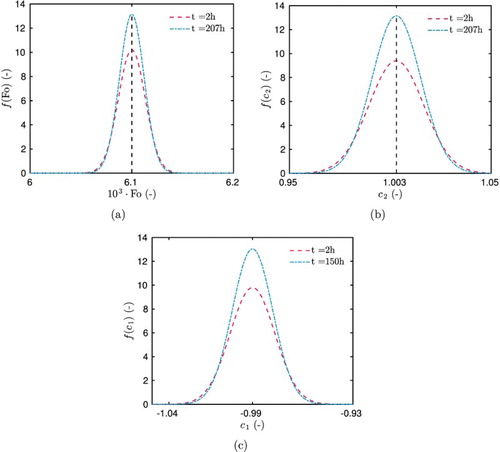
Figure 14. Variation of the criterion Ψ for the 16 possible designs for the adsorption coefficients (a) and the desorption coefficients (b).

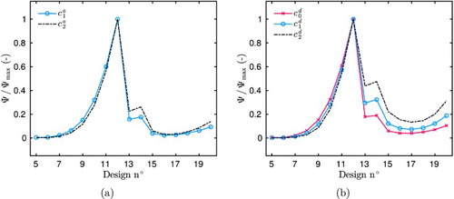
Figure 15. Sensitivity coefficients ${\mathrm{\Theta }}_u$ (a,b) and ${\mathrm{\Theta }}_c$ (c,d) for the OED (design 12, $X=X^{\circ }=1$).

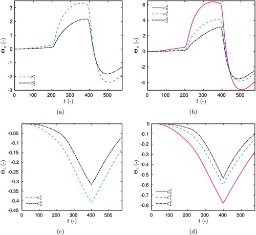
Figure 16. Sensitivity coefficients ${\mathrm{\Theta }}_u$ (a,b) and ${\mathrm{\Theta }}_c$ (c,d) for the design 20, ($X=X^{\circ }=1$).

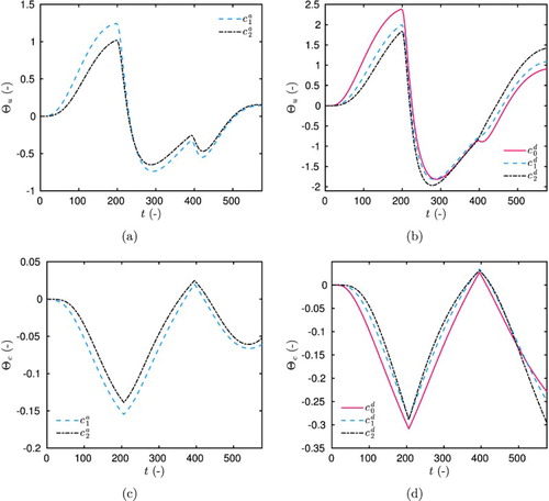
Table 4. Synthesis of OED for the estimation of one or several parameters when the model account for hysteresis.

		Optimal Experimental Design
	Parameter(s) to be estimated	Single-step	Multiple-step	Sensor position
One parameter	$c_{a,1}^{\star }$, $c_{a,2}^{\star }$, $c_{d,0}^{\star }$, $c_{d,1}^{\star }$ or $c_{d,2}^{\star }$	design 2	design 12	$X^{\circ }\in [0.85,1]$
Multiple parameter	$(c_{a,1}^{\star },c_{d,2}^{\star })$ or $(c_{a,2}^{\star },c_{d,2}^{\star })$	design 2	–	$X^{\circ }\in [0.85,1]$

Figure 17. Comparison of the numerical results with the experimental data (a) and their residual (b).

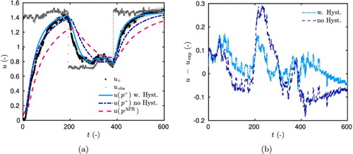
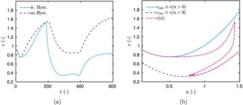
Figure 18. Variation of the sorption coefficient c according to time (a) and according to the computed field u (b).

Table

Latin letters
a	moisture advection coefficient ($\mathrm{s}/\mathrm{m}$)
$a_m$	mass transfer coefficient (${\mathrm{m}}^2/\mathrm{s}$)
c	moisture storage capacity ($\mathrm{kg}/({\mathrm{m}}^3.\mathrm{Pa})$)
$c_b$	specific heat $\left(\frac{\mathrm{J}}{\left(\mathrm{kg}.\mathrm{K}\right)}\right)$
d	moisture permeability (s)
h	convective vapour transfer coefficient ($\mathrm{s}/\mathrm{m}$)
L	length (m)
$P_s$	saturation pressure (Pa)
$P_v$	vapour pressure (Pa)
$r_{12}$	latent heat of evaporation (J/kg)
$R_v$	water gas constant (J/(kg.K))
T	temperature (K)
t	time coordinate (s)
U	relative moisture concentration (%)
x	space coordinate (m)
$\mathsf{v}$	mass average velocity (m/s)
w	specific moisture content(${\mathrm{kg}/\mathrm{m}}^3$)

Table

Greek letters
λ	thermal conductivity (W/(m.K))
δ	thermal-gradient coefficient (${\mathrm{K}}^{-1}$)
φ	relative humidity (-)
ρ	specific mass (${\mathrm{kg}/\mathrm{m}}^3$)

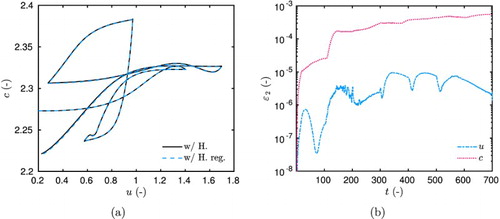
Figure A1. Time variation of the field u (a) and of the sorption capacity c (b) for the model with hysteresis and the regularised one.

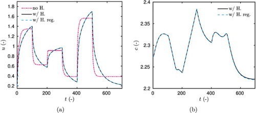
Figure A2. Variation of the sorption capacity c with the field u (a) according to the case study. Time variation of the ${\mathcal{L}}_2$ error (b) for the fields u and c between the model with hysteresis and the regularised one.

Berger J, Busser T, Dutykh D, et al. On the estimation of moisture permeability and advection coefficients of a wood fibre material using the optimal experiment design approach. Experiment Thermal and Fluid Sci. 2018;90.246–259. doi: 10.1016/j.expthermflusci.2017.07.026

 Web of Science ®Google Scholar

Rafidiarison H, Rémond R, Mougel E. Dataset for validating 1-d heat and mass transfer models within building walls with hygroscopic materials. Build Environ. 2015;89:356–368. doi: 10.1016/j.buildenv.2015.03.008

 Web of Science ®Google Scholar