Deep learning for photoacoustic tomography from sparse data

Figures & data

Figure 1. Basic principle of PAT. An object is illuminated with a short optical pulse (left) that induces an acoustic pressure wave (middle). The pressure signals are recorded outside of the object, and are used to recover an image of the interior (right).

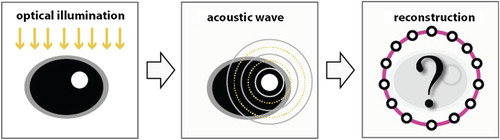
Figure 2. Illustration of the proposed network for PAT image reconstruction. In the first step, the FBP algorithm (or another standard linear reconstruction method) is applied to the sparse data. In a second step, a deep CNN is applied to the intermediate reconstruction which outputs an almost artefact-free image. This may be interpreted as a deep network with the FBP in the first layer and the CNN in the remaining layers.

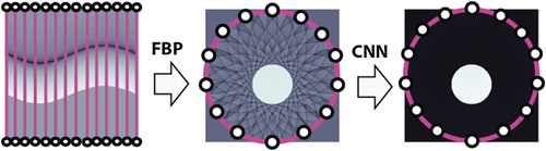
Figure 3. Sparse sampling problem in PAT in circular geometry. The induced acoustic pressure is measured at M detector locations on the boundary of the disc $B_R$ indicated by white dots in the left image. Every detector at location $z_m$ measures a time dependent pressure signal $\mathbf{p}[m,\cdot ]$, corresponding to a column in the right image.

Figure 4. Architecture of the used CNN (U-net with residual connection). The number written above each layer denotes the number of convolution kernels (channels), which is equal to number of images in each layer. The numbers $B_1,\dots ,B_5$ denote the dimension of the images (the block sizes in the weight matrices), which stays constant in every row. The long horizontal arrows indicate direct connections with subsequent concatenation or summation for the upmost arrow.

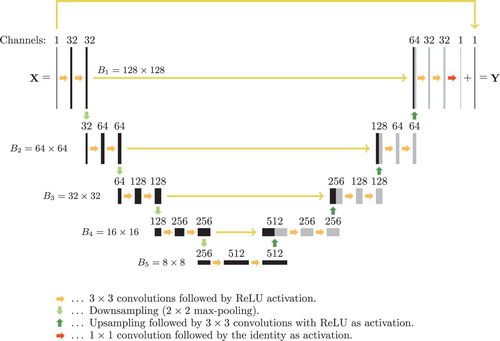
Figure 5. Results for simulated data (all images are displayed using the same colourmap). (a) Superposition of five ellipses as test phantom; (b) FBP reconstruction; (c) reconstruction using the proposed CNN; (d) TV reconstruction.

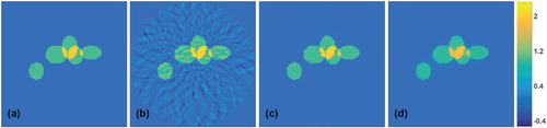
Table 1. Relative ${\ell }^2$-reconstruction errors for the four different test cases.

Phantom	FBP	TV	ELL	ELLn	SL	SLn
5 ellipses (exact)	0.1811	0.0144	0.0087	–	–	–
3 ellipses (noisy)	0.1952	0.0110	0.0051	0.0038	–	–
Shepp–Logan (exact)	0.3986	0.0139	0.1017	0.1013	0.0168	0.0186
Shepp–Logan (noisy)	0.3889	0.0154	0.1054	0.1027	0.0198	0.0206

Notes: Compared are FBP, TV, and the proposed CNN reconstruction trained on the class of ellipse phantoms without noise (ELL) and with noise (ELLn), as well as trained on a class containing Shepp–Logan type phantom without noise (SL) and with noise (SLn).

Figure 6. Results for noisy test data with 2% Gaussian noise added (all images are displayed using the same colourmap). (a) Reconstruction using the FBP algorithm; (b) reconstruction using the CNN trained without noise; (c) reconstruction using the CNN trained on noisy images; (d) TV reconstruction.

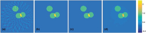
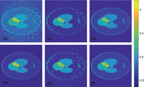
Figure 7. Reconstruction results for a Shepp–Logan type phantom using simultated data (all images are displayed using the same colourmap). (a) FBP reconstruction; (b) reconstruction using TV minimization. (c) Proposed CNN using wrong training data without noise added; (d) proposed CNN using wrong training data with noise added; (e) proposed CNN using appropriate training data without noise added; (f) proposed CNN using appropriate training data with noise added.

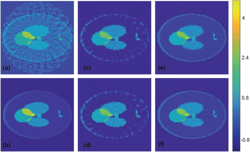
Figure 8. Reconstruction results for a Shepp–Logan type phantom from data with 2% Gaussian noise added (all images are displayed using the same colourmap). (a) FBP reconstruction; (b) reconstruction using TV minimization. (c) Proposed CNN using wrong training data without noise added; (d) proposed CNN using wrong training data with noise added; (e) proposed CNN using appropriate training data without noise added; (f) proposed CNN using appropriate training data with noise added.

Table 2. Average error analysis.

Phantom	FBP	TV	ELL	ELLn	SL	SLn
Exact	0.2188	0.0140	0.1218	0.1078	0.0215	0.0213
Noisy	0.2374	0.0150	0.1290	0.1141	0.0256	0.0243

Notes: Relative ${\ell }^2$-reconstruction error averaged of over 100 Shepp–Logan type phantoms. Compared are FBP, TV, proposed CNN reconstruction trained on a class of ellipse phantoms without noise (ELL) and with noise (ELLn), as well as trained on a class of containing Shepp–Logan type phantom without SL and with noise (SLn).