Figures & data
Figure 1. Schematic representation of the space bicomponent domain in two-dimensions.
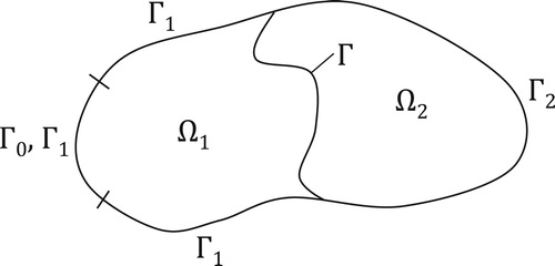
Figure 2. (a) The normalized objective functionalal , (b) the normalized accuracy error
, and (c) numerical solutions of
with initial guess
and
, for noise
, for Example 1.
![Figure 2. (a) The normalized objective functionalal J¯[φn], (b) the normalized accuracy error E¯[φn], and (c) numerical solutions of φ(t) with initial guess φ0(t)=0.5A and κ=1, for noise p∈{0,1,3}, for Example 1.](/cms/asset/b1e0c99a-01d5-4c9f-bae5-15697d78753b/gipe_a_1574781_f0002_ob.jpg)
Figure 3. Numerical solutions of for various values of the smoothing parameter
, with initial guess
, for (a) p=0, (b) p=1 and (c) p=3 noise, for Example 1.
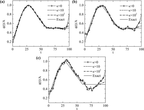
Figure 4. The normalized objective functionalal for (a)
and (b)
, and the normalized accuracy error
for (c)
and (d)
, for
noise, for Example 2.
![Figure 4. The normalized objective functionalal J¯[φn] for (a) κ=0 and (b) κ=103, and the normalized accuracy error E¯[φn] for (c) κ=0 and (d) κ=103, for p∈{0,3,5} noise, for Example 2.](/cms/asset/c0412a76-e2c2-44a9-94b9-6cba3e7eb4f1/gipe_a_1574781_f0004_ob.jpg)
Figure 5. Variation of the normalized accuracy error , at the stopping iteration number
, with respect to κ, for
noise, for Example 2.
![Figure 5. Variation of the normalized accuracy error E¯[φn], at the stopping iteration number ns, with respect to κ, for p∈{0,3,5} noise, for Example 2.](/cms/asset/acc1ef19-3cb0-4e8d-81f1-a3fb81da45ad/gipe_a_1574781_f0005_ob.jpg)
Figure 6. Retrieved solutions using various values of κ for (a) p=0, (b) p=3 and (c) p=5 noise, for Example 2.
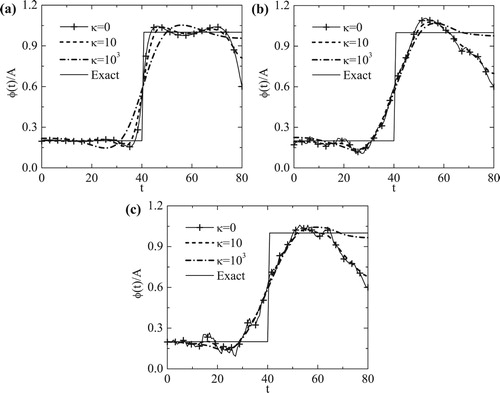
Figure 7. (a) The normalized objective functionalal and (b) the normalized accuracy error
for
, for
noise, for Example 3.
![Figure 7. (a) The normalized objective functionalal J¯[φn] and (b) the normalized accuracy error E¯[φn] for κ=1, for p∈{0,3,5} noise, for Example 3.](/cms/asset/2fa0f3c9-520d-4af1-9c2c-194a5f9e1d98/gipe_a_1574781_f0007_ob.jpg)
Figure 8. The variation of the normalized accuracy error with the smoothing parameter κ, for
noise, for Example 3.
![Figure 8. The variation of the normalized accuracy error E¯[φn] with the smoothing parameter κ, for p∈{0,3,5} noise, for Example 3.](/cms/asset/9de66707-55f2-467a-bd48-2c5200caecb3/gipe_a_1574781_f0008_ob.jpg)
Figure 9. (a) The exact given by (Equation45
(45)
(45) ) and the numerical solutions obtained with (b)
and (c)
after 40 iterations, for exact data (p=0), for Example 3.
![Figure 9. (a) The exact φ(y,t) given by (Equation45(45) φ⋆(y,t)=0.5AyLy+0.5AtT+0.1A,(y,t)∈[0,Ly]×[0,T],(45) ) and the numerical solutions obtained with (b) κ=0 and (c) κ=102 after 40 iterations, for exact data (p=0), for Example 3.](/cms/asset/18225f07-1534-47da-b094-245febb90b6a/gipe_a_1574781_f0009_ob.jpg)
Figure 10. The numerical solutions of for p=3 noise: (a)
, (b)
, and for p=5 noise: (c)
, (d)
, for Example 3.
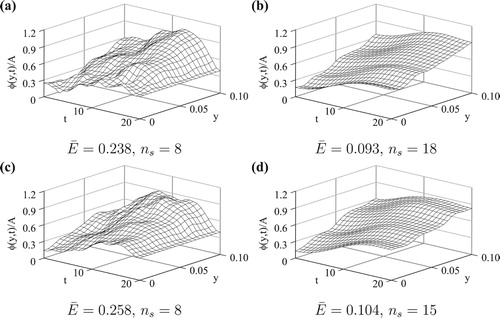
Figure 11. The variation of the normalized accuracy error , at the corresponding stopping iteration numbers, with the number of measurement points
, for
and p=5 noise, for Example 3.
![Figure 11. The variation of the normalized accuracy error E¯[φn], at the corresponding stopping iteration numbers, with the number of measurement points Nm, for κ∈{0,102} and p=5 noise, for Example 3.](/cms/asset/40888229-78a0-4f89-b9d7-e3433d96fb60/gipe_a_1574781_f0011_ob.jpg)
Figure 12. The variation of the normalized accuracy error with the smoothing parameter κ, for
noise, for Example 4.
![Figure 12. The variation of the normalized accuracy error E¯[φn] with the smoothing parameter κ, for p∈{0,3,5} noise, for Example 4.](/cms/asset/c40485d5-38f7-4588-b7cc-0e9e1abbd710/gipe_a_1574781_f0012_ob.jpg)
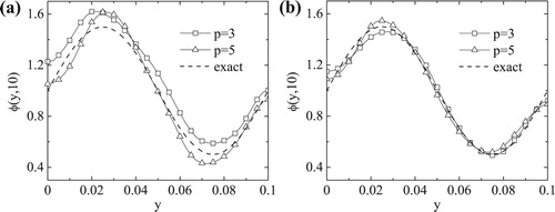
Figure 13. (a) The exact given by (Equation46
(46)
(46) ) and the numerical solutions obtained with (b)
and (c)
after 30 iterations, for exact data (p=0), for Example 4.
![Figure 13. (a) The exact φ(y,t) given by (Equation46(46) φ⋆(y,t)=0.5A⋅sin2πyLy+A,(y,t)∈[0,Ly]×[0,T],(46) ) and the numerical solutions obtained with (b) κ=0 and (c) κ=103 after 30 iterations, for exact data (p=0), for Example 4.](/cms/asset/be6be389-ff05-4453-86c9-af3d901f0222/gipe_a_1574781_f0013_ob.jpg)
Figure 14. The numerical solutions of for p=3 noise: (a)
, (b)
, and for p=5 noise: (c)
, (d)
, after
iterations, for Example 4.
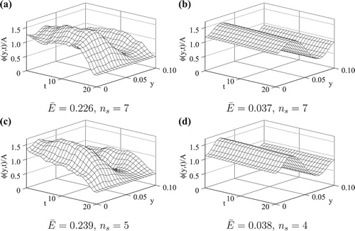
Figure 15. The exact and numerical solutions of for (a)
and (b)
after
iterations, for
noise, for Example 4.