Figures & data
Table 1. Parameter setup. We have used parameters and dimensions as described in [Citation9].
Figure 1. Uncertainty propagation. Subplots in the top row depict 100 perturbed samples of the thermal conductivity coefficient, given by Equation (Equation17(17)
(17) ), for
and
respectively. Subplots in the middle and the bottom rows depict the variance of the numerical simulation of forward mapping (Equation2
(2)
(2) ) acting on the above conductivity coefficients at r=0 and r=R respectively. The smoothing nature of the forward mapping makes it necessary to acquire temperature data at large integration times, e.g. 1000 s.
![Figure 1. Uncertainty propagation. Subplots in the top row depict 100 perturbed samples of the thermal conductivity coefficient, given by Equation (Equation17(17) k(t)=arctant30+0.45.(17) ), for SNR=10 and SNR=103 respectively. Subplots in the middle and the bottom rows depict the variance of the numerical simulation of forward mapping (Equation2(2) F(k)=T,(2) ) acting on the above conductivity coefficients at r=0 and r=R respectively. The smoothing nature of the forward mapping makes it necessary to acquire temperature data at large integration times, e.g. 1000 s.](/cms/asset/40cfca47-fb00-4f6e-a8bc-f7a141d3ed6a/gipe_a_1632841_f0001_ob.jpg)
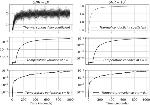
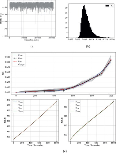
Figure 2. Example 1. (a) Trace plot. (b) Posterior distribution of . (c) True and estimators Middle row depicts 2000 samples of the posterior distribution of the thermal conductivity coefficient. At the bottom row are shown the corresponding temperatures evaluated at r=0 and r=R respectively. Hierarchical modelling.
![Figure 2. Example 1. (a) Trace plot. (b) Posterior distribution of σ2. (c) True and estimators Middle row depicts 2000 samples of the posterior distribution of the thermal conductivity coefficient. At the bottom row are shown the corresponding temperatures evaluated at r=0 and r=R respectively. Hierarchical modelling.](/cms/asset/33989c14-dbb6-4f12-a739-95b5fa77e8b0/gipe_a_1632841_f0002_oc.jpg)
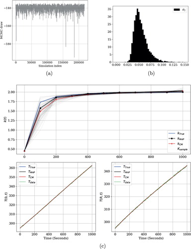
Figure 3. Example 2. (a) Trace plot. (b) Posterior distribution of . (c) True and estimators Middle row depicts 2000 samples of the posterior distribution of the thermal conductivity coefficient. At the bottom row are shown the corresponding temperatures evaluated at r=0 and r=R respectively. Hierarchical modelling.
![Figure 3. Example 2. (a) Trace plot. (b) Posterior distribution of σ2. (c) True and estimators Middle row depicts 2000 samples of the posterior distribution of the thermal conductivity coefficient. At the bottom row are shown the corresponding temperatures evaluated at r=0 and r=R respectively. Hierarchical modelling.](/cms/asset/336cb75d-c273-4f58-9486-3e3731bf06b9/gipe_a_1632841_f0003_oc.jpg)
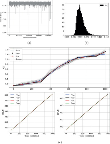
Figure 4. Example 3. (a) Trace plot. (b) Posterior distribution of . (c) True and estimators Middle row depicts 2000 samples of the posterior distribution of the thermal conductivity coefficient. At the bottom row are shown the corresponding temperatures evaluated at r=0 and r=R respectively. Hierarchical modelling.
![Figure 4. Example 3. (a) Trace plot. (b) Posterior distribution of σ2. (c) True and estimators Middle row depicts 2000 samples of the posterior distribution of the thermal conductivity coefficient. At the bottom row are shown the corresponding temperatures evaluated at r=0 and r=R respectively. Hierarchical modelling.](/cms/asset/5f54831c-cc3c-4acd-a09d-d1dedaf37733/gipe_a_1632841_f0004_oc.jpg)