Verification of sequential function specification method with intermittent spray cooling

Figures & data

Figure 1. Flow rate domain for continuous and intermittent sprays.

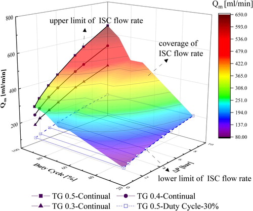
Figure 2. Schematic of the experimental system.

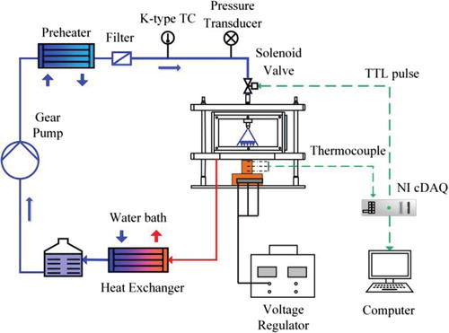
Table 1 Detailed information of experimental devices

Components	Manufacturer	Range
Nozzle	Spray System TG-0.4	1.5–10 bar
Data acquisition instrument	NI cDAQ 9212/9205	Maximum sample rate 95 Hz for temperature, 6.3 kHz for voltage
Geer Pump	Micro Pump PB23	For water:
		Max Diff-pressure: 8.7 bar
		Max flow rate:1000 ml/min
Solenoid valve	Parker Miniature Valves Series 9	Response time 6 ms, vac- 6.89 bar
Thermocouple	Omega GG-K-36	36 AWG, type-K
Pressure sensor	Danfoss AKS32	−1–12 bar
Cartridge heater	Omega CIR series	240 VAC, 500W

Figure 3. One-dimensional inverse heat conduction problem (not scaled, unit: mm): (a) copper block; (b) calculating domain.

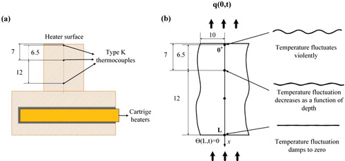
Figure 4. Illustration of the electronic control circuit for the solenoid valve.

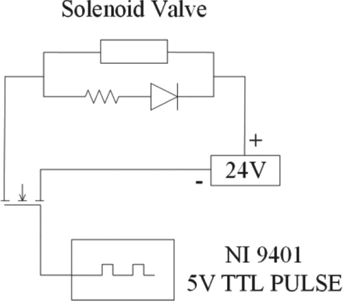
Figure 5. Calculated heat flux and temperature on the surface (using SFSM) where To = TL.

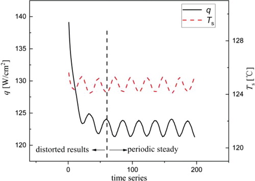
Table 2 Parameters of the numerical experiments.

	Regularization	Random noise [°C]	Time step [ms]	Injection duration [ms]	Period [ms]
Case 1	1,2,3,6	0.4	10	13	26
Case 2	2	0.4, 2	10	13	26
Case 3	2	0.4	1, 5, 10	13	26
Case 4	3, 6	0.4	1, 5, 10	165	330

Figure 6. Comparison between the exact and estimated heat flux (dt = 10 ms, T = 26 ms) for different regularization parameters r.

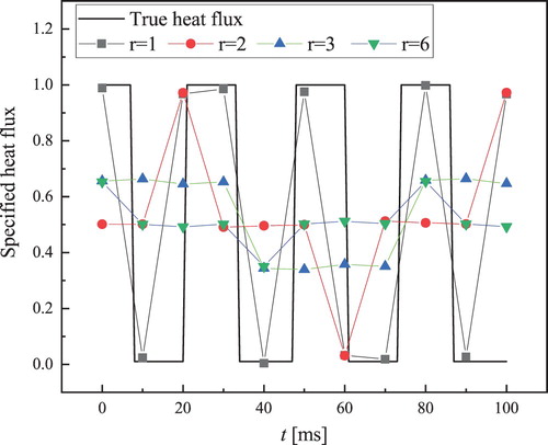
Figure 7. Comparison between exact and estimated heat flux (dt=10 ms, T=26 ms) for different random noises σ.

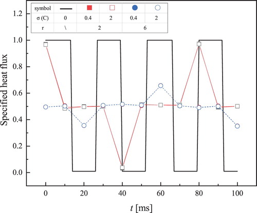
Figure 8. Comparison between exact and estimated heat flux (r = 2 ms, $\sigma$ = 0.4°C) for different time steps $\text{d}t$: (a) T = 26 ms; (b) T = 330 ms.

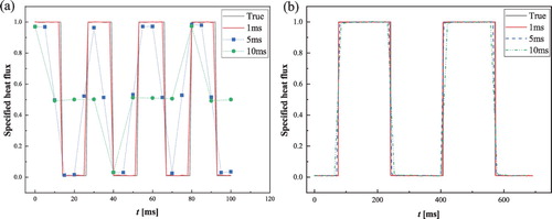
Figure 9. Comparison of standard deviation ${\sigma }_q$ versus bias B for different time steps $\text{d}t$ and pulse periods T.

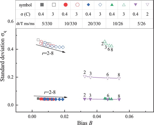
Figure 10. Typical fluctuations in control voltage, surface temperature, and heat flux at f = 2.5 Hz, DC = 80%, q = 122.8 W/cm² .

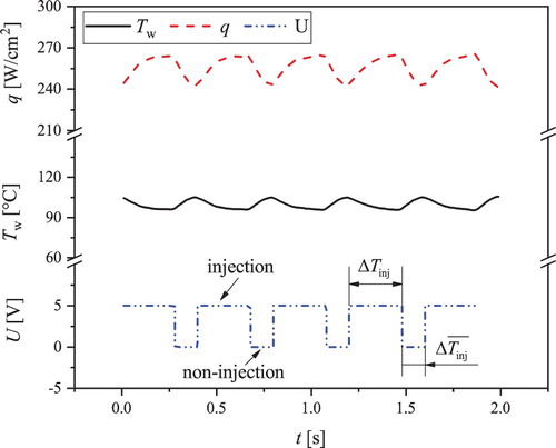
Figure 11. Calculated heat flux and heat transfer coefficient for r = 2, 3, 5, and 6, dt = 10.5 ms.

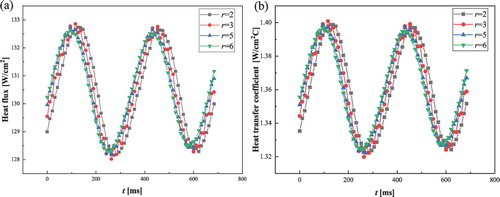
Figure 12. Transient behaviour of residual coolant on the heated surface in the non-injection duration ($\mathrm{\Delta }\overline{t_{\text{inj}}}$) at t′ = 0, t′ = 0.33, t′ = 0.66 and t′ = 1 $(t^{\mathrm{\prime }}=t/\mathrm{\Delta }\overline{t_{\text{inj}}})$.

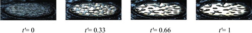
Figure 13. Calculated heat flux and heat transfer coefficient for dt = 10.5 and 21 ms with r = 3 and 6.

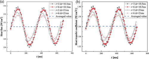
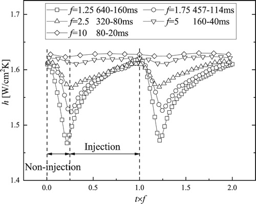
Figure 14. Heat transfer coefficient as a function of time with DC = 80%.