Improving a Tikhonov regularization method with a fractional-order differential operator for the inverse black body radiation problem

Figures & data

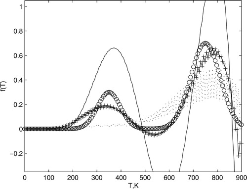
Figure 1. Comparison between exact (circle) and simulated (star) power spectrum radiated. The error bar represents the variation coefficient of $5\mathrm{\%}$, for values of ν between 0 and $1\times {10}^{14}$ Hz, and $10\mathrm{\%}$, for values of ν between $1\times {10}^{14}$ Hz and $2\times {10}^{14}$ Hz.

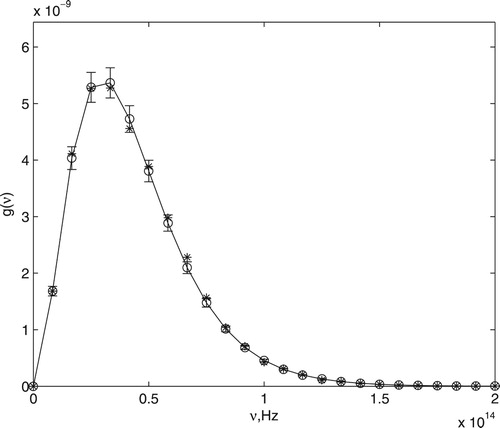
Figure 2. Comparison between exact (circle) and computed temperature distribution. The dotted line was obtained by Equation (2(2) $\begin{array}{rl}{\mathbf{f}}_{\lambda }& =\underset{\mathbf{f}}{min}{\varphi }_{\lambda }(\mathbf{f}),\\ {\mathbf{f}}_{\lambda }& =\{{\mathbf{K}}^T\mathbf{K}+{\lambda }^2(a_0{\mathbf{D}}^{(0)}+a_1{\mathbf{D}}^{(1)}+a_2{\mathbf{D}}^{(2)}){\}}^{-1}{\mathbf{K}}^T\mathbf{g}.\end{array}$(2) ) with $a_0=1$ and $a_1=a_2=0$ and continuous line by Equation (2(2) $\begin{array}{rl}{\mathbf{f}}_{\lambda }& =\underset{\mathbf{f}}{min}{\varphi }_{\lambda }(\mathbf{f}),\\ {\mathbf{f}}_{\lambda }& =\{{\mathbf{K}}^T\mathbf{K}+{\lambda }^2(a_0{\mathbf{D}}^{(0)}+a_1{\mathbf{D}}^{(1)}+a_2{\mathbf{D}}^{(2)}){\}}^{-1}{\mathbf{K}}^T\mathbf{g}.\end{array}$(2) ) with $a_1=1$ and $a_0=a_2=0$. Cross marker is the solution found by Equation (7(7) $\begin{array}{rl}{\mathbf{f}}_{\lambda ,\alpha }& =\underset{\mathbf{f}}{min}{\varphi }_{\lambda ,\alpha }(\mathbf{f}),\\ {\mathbf{f}}_{\lambda ,\alpha }& =\{{\mathbf{K}}^T\mathbf{K}+{\lambda }^2{\mathbf{D}}^{(\alpha )}{\}}^{-1}{\mathbf{K}}^T\mathbf{g},\end{array}$(7) ) with $\alpha =0.6$. All these results were obtained using $\lambda =3.16\times {10}^{-10}$.

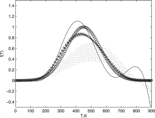
Figure 3. The L-curve for Equation (2(2) $\begin{array}{rl}{\mathbf{f}}_{\lambda }& =\underset{\mathbf{f}}{min}{\varphi }_{\lambda }(\mathbf{f}),\\ {\mathbf{f}}_{\lambda }& =\{{\mathbf{K}}^T\mathbf{K}+{\lambda }^2(a_0{\mathbf{D}}^{(0)}+a_1{\mathbf{D}}^{(1)}+a_2{\mathbf{D}}^{(2)}){\}}^{-1}{\mathbf{K}}^T\mathbf{g}.\end{array}$(2) ) with $a_0=1$ and $a_1=a_2=0$ (continuous line) and Equation (7(7) $\begin{array}{rl}{\mathbf{f}}_{\lambda ,\alpha }& =\underset{\mathbf{f}}{min}{\varphi }_{\lambda ,\alpha }(\mathbf{f}),\\ {\mathbf{f}}_{\lambda ,\alpha }& =\{{\mathbf{K}}^T\mathbf{K}+{\lambda }^2{\mathbf{D}}^{(\alpha )}{\}}^{-1}{\mathbf{K}}^T\mathbf{g},\end{array}$(7) ) with $\alpha =0.6$ (dotted line). The points marked by the square and the circle correspond to the regularization parameters of $3.16\times {10}^{-10}$ using Equations (2(2) $\begin{array}{rl}{\mathbf{f}}_{\lambda }& =\underset{\mathbf{f}}{min}{\varphi }_{\lambda }(\mathbf{f}),\\ {\mathbf{f}}_{\lambda }& =\{{\mathbf{K}}^T\mathbf{K}+{\lambda }^2(a_0{\mathbf{D}}^{(0)}+a_1{\mathbf{D}}^{(1)}+a_2{\mathbf{D}}^{(2)}){\}}^{-1}{\mathbf{K}}^T\mathbf{g}.\end{array}$(2) ) and (7(7) $\begin{array}{rl}{\mathbf{f}}_{\lambda ,\alpha }& =\underset{\mathbf{f}}{min}{\varphi }_{\lambda ,\alpha }(\mathbf{f}),\\ {\mathbf{f}}_{\lambda ,\alpha }& =\{{\mathbf{K}}^T\mathbf{K}+{\lambda }^2{\mathbf{D}}^{(\alpha )}{\}}^{-1}{\mathbf{K}}^T\mathbf{g},\end{array}$(7) ), respectively. The result obtained by $1.26\times {10}^{-9}$ and $\alpha =0.6$ is shown by triangle symbol.

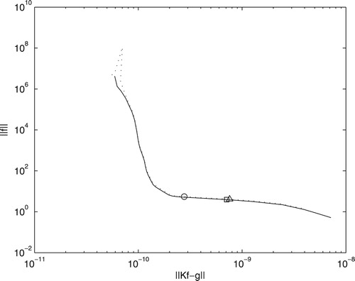
Figure 4. Comparison between exact (circle) and two computed temperature distribution. Cross marker is the solution found by Equation (7(7) $\begin{array}{rl}{\mathbf{f}}_{\lambda ,\alpha }& =\underset{\mathbf{f}}{min}{\varphi }_{\lambda ,\alpha }(\mathbf{f}),\\ {\mathbf{f}}_{\lambda ,\alpha }& =\{{\mathbf{K}}^T\mathbf{K}+{\lambda }^2{\mathbf{D}}^{(\alpha )}{\}}^{-1}{\mathbf{K}}^T\mathbf{g},\end{array}$(7) ) with $\alpha =0.6$ and $\lambda =3.16\times {10}^{-10}$. Triangle marker is the solution found by Equation (7(7) $\begin{array}{rl}{\mathbf{f}}_{\lambda ,\alpha }& =\underset{\mathbf{f}}{min}{\varphi }_{\lambda ,\alpha }(\mathbf{f}),\\ {\mathbf{f}}_{\lambda ,\alpha }& =\{{\mathbf{K}}^T\mathbf{K}+{\lambda }^2{\mathbf{D}}^{(\alpha )}{\}}^{-1}{\mathbf{K}}^T\mathbf{g},\end{array}$(7) ) with $\alpha =0.6$ and $\lambda =1.26\times {10}^{-9}$.

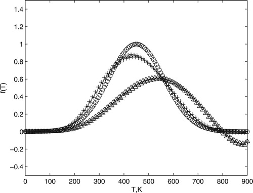
Figure 5. The exact temperature distribution (circle) and the results obtained with $25\times 150$ dimension of the matrix K (star) and $25\times 300$ dimension of the matrix K (triangle). All these results were obtained using $\lambda =3.16\times {10}^{-10}$ and $\alpha =0.6$.

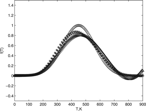
Figure 6. The Euclidian norm of the first-order derivative of the solution obtained by Equation (7(7) $\begin{array}{rl}{\mathbf{f}}_{\lambda ,\alpha }& =\underset{\mathbf{f}}{min}{\varphi }_{\lambda ,\alpha }(\mathbf{f}),\\ {\mathbf{f}}_{\lambda ,\alpha }& =\{{\mathbf{K}}^T\mathbf{K}+{\lambda }^2{\mathbf{D}}^{(\alpha )}{\}}^{-1}{\mathbf{K}}^T\mathbf{g},\end{array}$(7) ) for different values of α, at fixed λ.

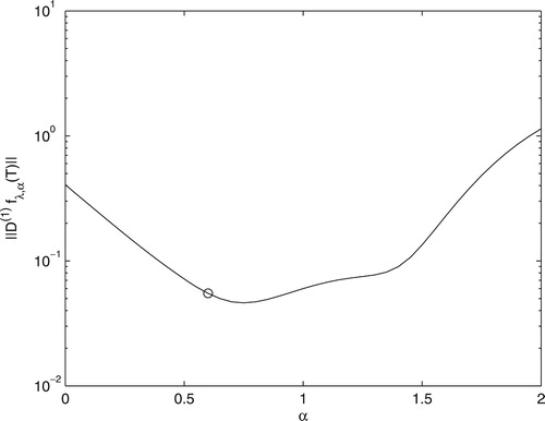
Figure 7. The triangle represents the residual to the result obtained by Equation (2(2) $\begin{array}{rl}{\mathbf{f}}_{\lambda }& =\underset{\mathbf{f}}{min}{\varphi }_{\lambda }(\mathbf{f}),\\ {\mathbf{f}}_{\lambda }& =\{{\mathbf{K}}^T\mathbf{K}+{\lambda }^2(a_0{\mathbf{D}}^{(0)}+a_1{\mathbf{D}}^{(1)}+a_2{\mathbf{D}}^{(2)}){\}}^{-1}{\mathbf{K}}^T\mathbf{g}.\end{array}$(2) ) with $a_0=1$ and $a_1=a_2=0$ and the circle represents the residual to the result obtained by Equation (2(2) $\begin{array}{rl}{\mathbf{f}}_{\lambda }& =\underset{\mathbf{f}}{min}{\varphi }_{\lambda }(\mathbf{f}),\\ {\mathbf{f}}_{\lambda }& =\{{\mathbf{K}}^T\mathbf{K}+{\lambda }^2(a_0{\mathbf{D}}^{(0)}+a_1{\mathbf{D}}^{(1)}+a_2{\mathbf{D}}^{(2)}){\}}^{-1}{\mathbf{K}}^T\mathbf{g}.\end{array}$(2) ) with $a_1=1$ and $a_0=a_2=0$. The square is the result to Equation (7(7) $\begin{array}{rl}{\mathbf{f}}_{\lambda ,\alpha }& =\underset{\mathbf{f}}{min}{\varphi }_{\lambda ,\alpha }(\mathbf{f}),\\ {\mathbf{f}}_{\lambda ,\alpha }& =\{{\mathbf{K}}^T\mathbf{K}+{\lambda }^2{\mathbf{D}}^{(\alpha )}{\}}^{-1}{\mathbf{K}}^T\mathbf{g},\end{array}$(7) ) with $\alpha =0.6$. The error bar represents the variation coefficient of $5\mathrm{\%}$, for values of ν between 0 and $1\times {10}^{14}$ Hz, and $10\mathrm{\%}$, for values of ν between $1\times {10}^{14}$ and $2\times {10}^{14}$ Hz.

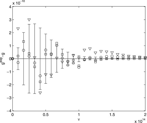
Figure 8. The exact temperature distribution (Equation (14(14) $\begin{array}{rl}f(T)& =\frac{\tanh \left(\frac{T-250}{20}\right)+\tanh \left(\frac{-T+550}{20}\right)}{2},\end{array}$(14) )) is shown with circle marker and compared to different computed results. The dotted line was obtained by Equation (2(2) $\begin{array}{rl}{\mathbf{f}}_{\lambda }& =\underset{\mathbf{f}}{min}{\varphi }_{\lambda }(\mathbf{f}),\\ {\mathbf{f}}_{\lambda }& =\{{\mathbf{K}}^T\mathbf{K}+{\lambda }^2(a_0{\mathbf{D}}^{(0)}+a_1{\mathbf{D}}^{(1)}+a_2{\mathbf{D}}^{(2)}){\}}^{-1}{\mathbf{K}}^T\mathbf{g}.\end{array}$(2) ) with $a_0=1$ and $a_1=a_2=0$ and continuous line by Equation (2(2) $\begin{array}{rl}{\mathbf{f}}_{\lambda }& =\underset{\mathbf{f}}{min}{\varphi }_{\lambda }(\mathbf{f}),\\ {\mathbf{f}}_{\lambda }& =\{{\mathbf{K}}^T\mathbf{K}+{\lambda }^2(a_0{\mathbf{D}}^{(0)}+a_1{\mathbf{D}}^{(1)}+a_2{\mathbf{D}}^{(2)}){\}}^{-1}{\mathbf{K}}^T\mathbf{g}.\end{array}$(2) ) with $a_1=1$ and $a_0=a_2=0$. Cross marker is the solution found by Equation (7(7) $\begin{array}{rl}{\mathbf{f}}_{\lambda ,\alpha }& =\underset{\mathbf{f}}{min}{\varphi }_{\lambda ,\alpha }(\mathbf{f}),\\ {\mathbf{f}}_{\lambda ,\alpha }& =\{{\mathbf{K}}^T\mathbf{K}+{\lambda }^2{\mathbf{D}}^{(\alpha )}{\}}^{-1}{\mathbf{K}}^T\mathbf{g},\end{array}$(7) ) with $\alpha =0.6$. All these results were obtained using $\lambda =1.95\times {10}^{-10}$.

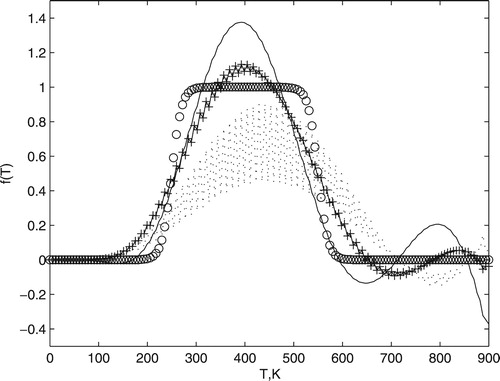
Figure 9. The circle marker is the exact temperature distribution (Equation (15(15) $\begin{array}{rl}f(T)& =0.3\exp \left(\frac{-(T-350{)}^2}{4500}\right)+0.7\exp \left(\frac{-(T-750{)}^2}{7500}\right).\end{array}$(15) )). The dotted line was obtained by Equation (2(2) $\begin{array}{rl}{\mathbf{f}}_{\lambda }& =\underset{\mathbf{f}}{min}{\varphi }_{\lambda }(\mathbf{f}),\\ {\mathbf{f}}_{\lambda }& =\{{\mathbf{K}}^T\mathbf{K}+{\lambda }^2(a_0{\mathbf{D}}^{(0)}+a_1{\mathbf{D}}^{(1)}+a_2{\mathbf{D}}^{(2)}){\}}^{-1}{\mathbf{K}}^T\mathbf{g}.\end{array}$(2) ) with $a_0=1$ and $a_1=a_2=0$ and continuous line by Equation (2(2) $\begin{array}{rl}{\mathbf{f}}_{\lambda }& =\underset{\mathbf{f}}{min}{\varphi }_{\lambda }(\mathbf{f}),\\ {\mathbf{f}}_{\lambda }& =\{{\mathbf{K}}^T\mathbf{K}+{\lambda }^2(a_0{\mathbf{D}}^{(0)}+a_1{\mathbf{D}}^{(1)}+a_2{\mathbf{D}}^{(2)}){\}}^{-1}{\mathbf{K}}^T\mathbf{g}.\end{array}$(2) ) with $a_1=1$ and $a_0=a_2=0$. Cross marker is the solution found by Equation (7(7) $\begin{array}{rl}{\mathbf{f}}_{\lambda ,\alpha }& =\underset{\mathbf{f}}{min}{\varphi }_{\lambda ,\alpha }(\mathbf{f}),\\ {\mathbf{f}}_{\lambda ,\alpha }& =\{{\mathbf{K}}^T\mathbf{K}+{\lambda }^2{\mathbf{D}}^{(\alpha )}{\}}^{-1}{\mathbf{K}}^T\mathbf{g},\end{array}$(7) ) with $\alpha =0.6$. All these results were achieved using $\lambda =4.47\times {10}^{-10}$.