A reconstruction of object properties with significant uncertainties

Figures & data

Figure 1. Typical behaviour of the solutions to the direct problem (9) – (11).

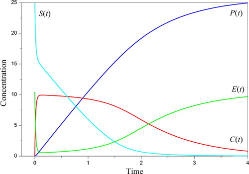
Figure 2. Invariant I₁ of the problem (9) – (11) with the parameters (23): 1 – $I_1^{(1)}=\frac{10t}{2t^2-5t+4}$; 2 – $I_1^{(2)}=-0.1t(t-20)$; 3 – $I_1^{(3)}=\frac{15t}{t+50\exp (-t)}$; 4 – $I_1^{(4)}=\frac{2.95t}{1+0.01\exp (0.05t^2)}$.

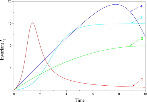
Figure 3. Invariant I₂ = S(I₁/C – 1) of the problem (9) – (11) with the parameters (23) and various I₁: 1 – $I_1^{(1)}=\frac{10t}{2t^2-5t+4}$; 2 – $I_1^{(2)}=-0.1t(t-20)$; 3 – $I_1^{(3)}=\frac{15t}{t+50\exp (-t)}$; 4 – $I_1^{(4)}=\frac{2.95t}{1+0.01\exp (0.05t^2)}$.

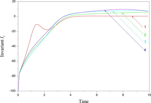
Figure 4. The parameters k_-1 from the invariant subset (18): 1 – the parent function from (23), 2 – transformed by$I_2^{(1)}$, 3 – transformed by $I_2^{(2)}$, 4 – transformed by $I_2^{(3)}$, 5 – transformed by $I_2^{(4)}$.

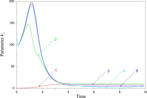
Figure 5. The parameters k₁ from the invariant subset (19): 1 – the parent function from (23), 2 – transformed by $I_1^{(1)}$, 3 – transformed by $I_1^{(2)}$, 4 – transformed by $I_1^{(3)}$, 5 – transformed by $I_1^{(4)}$.

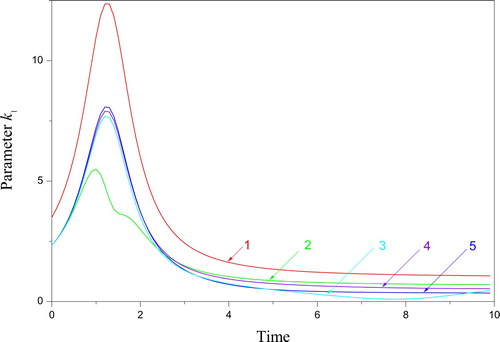
Figure 6. The possibility of matching two different hyperbolas.

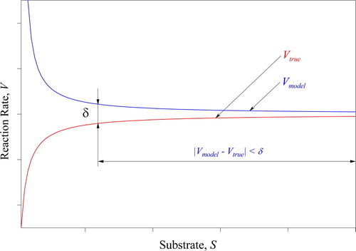
Table 1. The reconstruction $\{a,T_{obs}\}$ for the experimental data [55].

				The constant parameters {k-1, k1, k2, S0, E0} = const						The piecewise linear functions $\{k_{-1},k_1,k_2{\}}_N$ and S0, E0 = const
	The samples		2. Sub- problem (28)	3.1. Subproblem (24)			3.2. Subproblem (26), (27) ${\hat{\delta }}_1=0.0048,{\hat{\delta }}_2=0.0031$			4.1. Subproblem (26), (27), N=9, ${\hat{\delta }}_1={0.1}_{{10}^{-4}},{\hat{\delta }}_2={0.322}_{{10}^{-4}}$			4.2. Subproblem (26), (27), N = 66 ${\hat{\delta }}_1={0.193}_{{10}^{-4}},{\hat{\delta }}_2={0.322}_{{10}^{-4}}$
	$S_{}^{(\delta )}$	$V_{}^{(\delta )}$	$V_{}^{(\delta )}$-V	Tobs	$S_{}^{(\delta )}$- S	$V_{}^{(\delta )}$-V	Tobs	$S_{}^{(\delta )}$- S	$V_{}^{(\delta )}$-V	Tobs	$S_{}^{(\delta )}$- S	$V_{}^{(\delta )}$-V	Tobs	$S_{}^{(\delta )}$- S	$V_{}^{(\delta )}$-V
1	1.078	0.445	−0.001133	1.24229	0.110−^12	0.79410−^2	0.63633	0.002	−0.72710−^3	0.65044	−0.210−^4	−0.32210−^4	0.62546	0.00001	−0.32210−^4
2	0.647	0.435	0.007837	2.42073	0.210−^12	0.13110−^2	1.71704	0.001	−0.30710−^2	1.70809	0.210−^4	0.58310−^5	1.68525	0.00001	0.38010−^5
3	0.431	0.400	−0.005547	3.32786	0.110−^12	0.75610−^2	2.51022	−0.005	0.31110−^2	2.48007	0.110−^5	0.17310−^4	2.45635	0.00001	0.17010−^5
4	0.216	0.345	−0.007382	4.80068	0.110−^12	0.36110−^2	3.66652	−0.005	0.48110−^3	3.67470	0.110−^5	−0.61810−^6	3.62732	0.00000	0.51310−^6
5	0.129	0.305	0.005669	5.99937	0.210−^12	−0.79210−^2	4.41861	0.005	−0.31010−^2	4.51807	0.110−^4	−0.54610−^6	4.46809	0.00000	0.66110−^6
6	0.086	0.260	0.007389	7.11076	0.210−^12	−0.79410−^2	5.19856	0.001	−0.30910−^2	5.24427	0.210−^6	−0.86910−^6	5.18027	0.00000	0.48810−^5
7	0.050	0.180	−0.008189	8.98218	0.510−^12	0.79810−^2	6.67817	−0.005	0.31010−^2	6.43897	0.510−^6	−0.10810−^5	6.39092	−0.00002	0.69910−^5
8	0.040	0.165	0.001581	9.87074	0.210−^12	−0.20410−^2	7.03681	−0.001	0.31010−^2	6.97660	0.210−^6	0.12410−^5	6.91641	0.00002	0.98010−^6
9	0.030	0.140	0.005981	11.1110	0.110−^12	−0.67810−^2	7.70444	0.001	0.31010−^2	7.72943	0.110−^6	−0.14610−^5	7.64525	0.00001	0.90110−^5

Table 2. The measure of the solution complexity and matching with the observations for the different number of nodes N, experimental data [55], and subproblem (26), (27).

The number of nodes, N	9	25	34	44	50	60	66
${\displaystyle \int {\left({\displaystyle \frac{d{k}_1}{dt}}\right)}^{2}dt+\int {\left({\displaystyle \frac{d{k}_{-1}}{dt}}\right)}^{2}dt+\int {\left({\displaystyle \frac{d{k}_2}{dt}}\right)}^{2}dt}$	0.071665	0.051513	0.051046	0.048140	0.039877	0.025544	0.013569
$\underset{1\le i\le m}{\text{max}}|S{(t_i)|}_{a^{(\delta )}}-S_i^{(\delta )}|$	0.2390810−^4	0.1876210−^4	0.22710−^10	0.22710−^10	0.22710−^10	0.1784910−^4	0.1927410−^4
${\displaystyle \sum _{i=1}^m[S{(t_i)|}_a-S_i^{(\delta )}{]}^2}$	0.9846610−^5	0.1035210−^4	0.11110−^10	0.11110−^10	0.11110−^10	0.9313410−^5	0.1074910−^4
$\underset{1\le i\le m}{\text{max}}|V{(t_i)|}_{a^{(\delta )}}-V_i^{(\delta )}|$	0.3211110−^4	0.1751710−^4	0.11410−^4	0.77510−^5	0.13010−^4	0.1987810−^4	0.3212610−^4
${\displaystyle \sum _{i=1}^m[V{(t_i)|}_{\hat{a}}-V_i^{(\delta )}{]}^2}$	0.1234610−^4	0.1093110−^4	0.36310−^5	0.31310−^5	0.64110−^5	0.1116010−^4	0.1157210−^4

Table 3. The reconstruction $\{a,T_{obs}\}$ for the experimental data [56].

				3. The piecewise constant functions $\{k_{-1},k_1,k_2{\}}_{N=3}$ and S0, E0=const, subproblem (26), (27) ${\hat{\delta }}_1=0.0003,{\hat{\delta }}_2=0.129$							4. The piecewise linear functions $\{k_{-1},k_1,k_2{\}}_N$ and S0, E0 = const
	1. The samples		2. Subproblem (28)	4.1. Subproblem (24), N = 6		4.2. Subproblem (24), N = 11			4.3. Subproblem (24), N = 31			4.4. Subproblem (24), N = 51			4.5. Subproblem (26), (27), N = 176, ${\hat{\delta }}_1=0.0005,{\hat{\delta }}_2=0.001$
	$S_{}^{(\delta )}$	$V_{}^{(\delta )}$	$V_{}^{(\delta )}$-V	Tobs	$S_{}^{(\delta )}$- S	$V_{}^{(\delta )}$-V	Tobs	$V_{}^{(\delta )}$-V	Tobs	$V_{}^{(\delta )}$-V	Tobs	$V_{}^{(\delta )}$-V	Tobs	$V_{}^{(\delta )}$-V	Tobs	$S_{}^{(\delta )}$- S	$V_{}^{(\delta )}$-V
1	67.60	0.997	−0.18826	0.00641	0.29710−^3	−0.16410−^2	1.1965	0.69610−^3	1.1952	0.47010−^3	1.2003	−0.11310−^4	1.2003	−0.50210−^5	1.190	−0.00038	−0.10910−^2
2	29.514	0.990	−0.07694	32.31156	−0.34210−^3	−0.126	40.737	0.10810−^2	40.725	−0.15310−^3	39.987	−0.20110−^5	39.988	−0.18410−^5	39.513	0.00045	0.10910−^2
3	12.88	0.969	0.10075	48.39442	0.15010−^3	0.22210−^1	57.511	−0.48710−^2	57.534	−0.17510−^3	57.179	0.20510−^7	57.181	0.15110−^5	56.673	−0.00049	−0.10910−2
4	7.940	0.909	0.18880	54.17396	0.19910−^3	0.97910−^1	62.845	0.39610−^2	62.882	0.44410−^4	62.517	−0.12210−^6	62.518	−0.91110−^6	62.042	−0.00049	0.11210−3
5	5.750	0.760	0.14409	57.21288	0.18710−^3	0.49810−^1	65.550	0.10310−^3	65.589	−0.18310−^3	65.240	−0.10510−^5	65.242	−0.77510−^5	64.858	−0.00050	0.42210−4
6	4.467	0.500	−0.03520	59.27994	0.15610−^3	−0.128	67.981	0.12810−^3	68.026	0.14310−^3	67.685	0.22110−^6	67.686	−0.20410−^5	67.161	−0.00051	−0.25910−3
7	2.884	0.240	−0.16474	65.01216	−0.29710−^3	−0.51310−^3	74.305	0.87410−^4	74.331	−0.19610−^3	74.382	−0.88310−^7	74.312	0.33910−^5	72.349	−0.00050	−0.84110−^4
8	1.748	0.0909	−0.18880	78.77295	−0.30810−^3	0.80110−^2	81.320	0.69010−^4	81.273	0.60110−^4	80.995	0.17610−^5	81.145	0.26310−^6	80.565	−0.00050	−0.49910−^4
9	0.794	0.0306	−0.11340	96.59349	−0.24410−^3	−0.10210−^1	124.548	0.15110−^2	162.975	−0.42710−^5	170.693	0.13810−^6	174.821	−0.11710−^7	99.382	−0.00050	0.13010−^3
10	0.350	0.0099	−0.57779	114.2763	−0.14510−^3	−0.88210−^2	147.628	−0.30810−^2	182.562	−0.15110−^3	198.263	−0.26910−^5	203.229	−0.44610−^6	124.183	−0.00050	0.32910−^5
11	0.100	0.00315	−0.01694	140.6856	−0.54210−^4	−0.23210−^2	182.617	−0.58510−^3	227.377	0.26310−^3	241.129	0.23210−^6	245.464	0.25210−^6	157.756	0.00021	0.10810−^2

Table 4. The measure of the solution complexity and matching with the observations for the different number of nodes N, experimental data [56], and subproblem (24).

The number of nodes N	6	11	31	51	71	91	101	176
${\displaystyle \int {\left({\displaystyle \frac{d{k}_1}{dt}}\right)}^{2}dt+\int {\left({\displaystyle \frac{d{k}_{-1}}{dt}}\right)}^{2}dt+\int {\left({\displaystyle \frac{d{k}_2}{dt}}\right)}^{2}dt}$	521.5505	309.388	238.5441	134.4317	60.3046	24.3784	22.0499	9.9679
$\underset{1\le i\le m}{\text{max}}|S{(t_i)|}_{a^{(\delta )}}-S_i^{(\delta )}|$	0.22710−^10	0.45410−^9	0.22710−^10	0.22710−^10	0.22710−^10	0.22710−^10	0.22710−^10	0.50510−^3
${\displaystyle \sum _{i=1}^m[S{(t_i)|}_a-S_i^{(\delta )}{]}^2}$	0.10410−^10	0.17910−^9	0.11110−^10	0.11110−^10	0.11110−^10	0.11110−^10	0.11110−^10	0.46610−^3
$\underset{1\le i\le m}{\text{max}}|V{(t_i)|}_{a^{(\delta )}}-V_i^{(\delta )}|$	0.48710−^2	0.47010−^3	0.11410−^4	0.77510−^5	0.13010−^4	0.33610−^4	0.44110−^4	0.10910−^2
${\displaystyle \sum _{i=1}^m[V{(t_i)|}_{\hat{a}}-V_i^{(\delta )}{]}^2}$	0.22110−^2	0.22010−^3	0.36310−^5	0.31310−^5	0.64110−^5	0.15710−^4	0.14610−^4	0.66410−^3

Figure 7. The estimation of the parameter k_-1 for the various nodes N (its value is indicated on the curves).

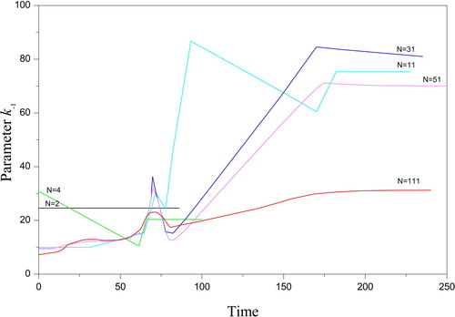
Figure 8. The estimation of the parameter k₁ for the various nodes N (its value is indicated on the curves).

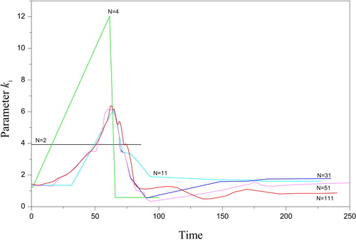
Figure 9. The estimation of the parameter k₂ for the various nodes N (its value is indicated on the curves).

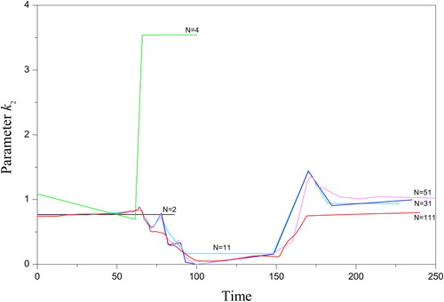
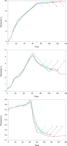
Figure 10. The reconstructed kinetic parameters, N = 176 (the experimental data [56]): 1 – the parameter k_-1, 2 – the parameter k₁, 3 – the parameter k₂.

Figure 11. The reconstructed functions, N = 176 (the experimental data [56]): 1 – C, 2 – V.

Figure 12. The dependence V(S): 1 – the experimental data [56], 2 – the regularized solution, N = 176, 3 – the Michaelis-Menten function with the parameters $V_{max}^{(0)}$ and $K_M^{(0)}$.

Figure 13. The exclusion of the locally sequential refinement from the sequence (24) – (27), N = 11.

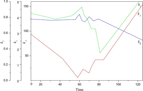
Figure 14. The local refinement without the regularization, N = 71.

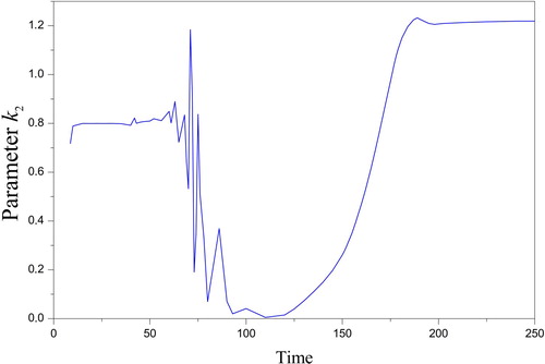
Figure 15. The magnification of nodes and the local violation of the function V monotonous: a) N = 95; b) N = 131; c) N = 161; d) N = 95; e) N = 131; f) N = 151.

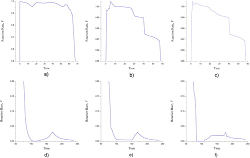
Figure 16. The sample simulation with the noise level 1%, 5% and 10%.

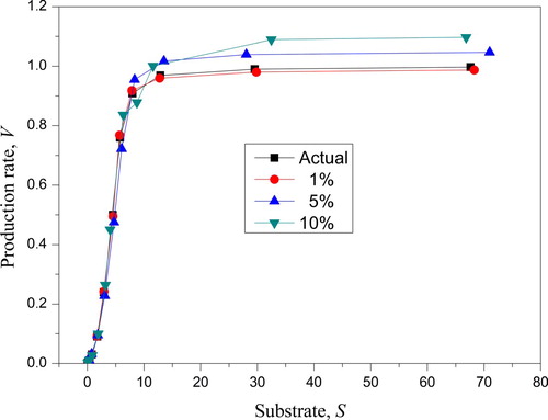
Figure 17. The reconstruction with the noise simulation: 1 – the actual parameter, 2 – the noise level 1%, 3 – the noise level 5%, 4 – the noise level 10%.

Hanes CS. The effect of starch concentration upon the velocity of hydrolysis by the amylase of germinated barley. Biochem J. 1932;26(5):1406–1421. doi: 10.1042/bj0261406

 Google Scholar

Dette H, Melas VB, Wong WK. Optimal design for goodness-of-fit of the Michaelis–Menten enzyme kinetic function. J Am Stat Assoc. 2005;100(472):1370–1381. doi: 10.1198/016214505000000600

 Google Scholar