Applying the solotone inverse method to estimate thermophysical properties of bonds and to locate internal boundaries, including regions of porosity

Figures & data

Figure 1. Schematic of a solid composite rod showing discontinuities in the heat capacity c and thermal conductivity k.

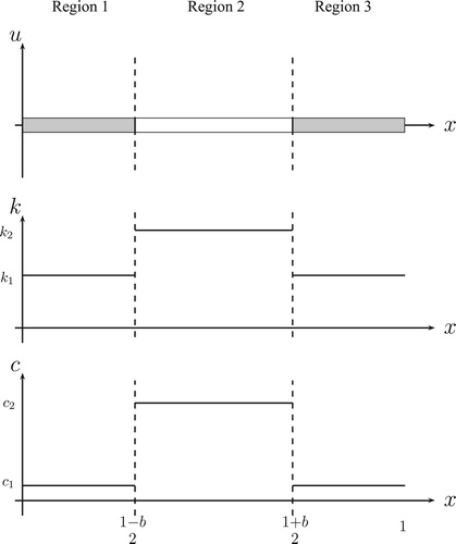
Figure 2. Schematic of a solid composite rod showing a narrow central bond or weld.

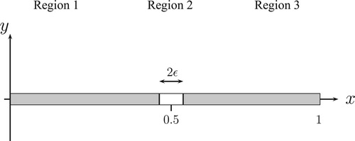
Figure 3. One possible distribution of eigenvalues for a rod with a very narrow central section.

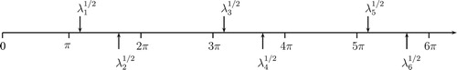
Figure 4. Variation in solotone period for $ϵ=0.0025$, representing a bond width of 0.5%. The values of γ are: 0.01, 0.1, 0.5, 1.0, 2.5, 5.0, 7.5, 10.0.

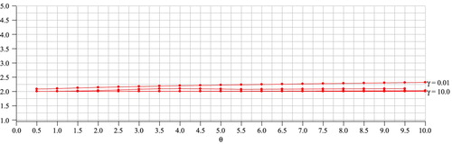
Figure 5. Variation in solotone period for $ϵ=0.025$, representing a bond width of 5%.

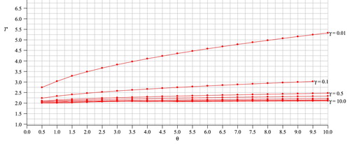
Figure 6. Variation in solotone period for $ϵ=0.05$, representing a bond width of 10%. The horizontal dashed line shows the solotone period for a steel–epoxyadhesive–steel rod.

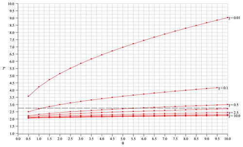
Table 1. Solotone period as a function of bond width for a steel–epoxyadhesive–steel rod.

Bond Width	Bond Width (%)	Solotone Period
0.0025	0.5	2.0082
0.0050	1.0	2.0913
0.0100	2.0	2.1401
0.0150	3.0	2.2104
0.0200	4.0	2.2829
0.0250	5.0	2.3571
0.0375	7.5	2.5498
0.0500	10.0	2.7532

Table 2. Thermal conductivity $k_{1,2}$, specific heat capacity $c_{1,2}$, and relative discontinuities $k_2/k_1$ and $c_2/c_1$ for steel and epoxy adhesive.

Steel	Epoxy Adhesive	Relative Discontinuities
$k_1=33.5$	$k_2=1.84$	$\gamma =0.055$
$c_1=475$	$c_2=300$	$\theta =0.632$

Figure 7. Variation in Euclidean distance for $ϵ=0.05$. The horizontal dashed line shows the Euclidean distance for a steel–epoxyadhesive–steel rod.

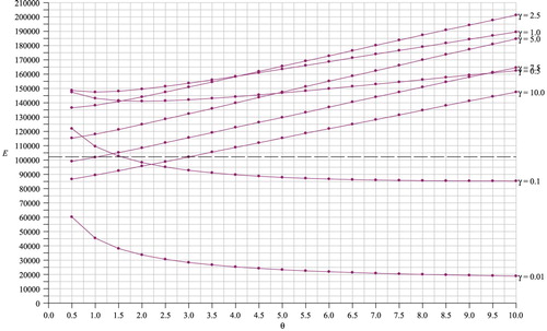
Figure 8. Variation in solotone period for $ϵ=0.05$ (finer scale). The horizontal lines of short dashes show $T^{\prime }\pm 1\mathrm{\%}$ for a steel–epoxyadhesive–steel rod.

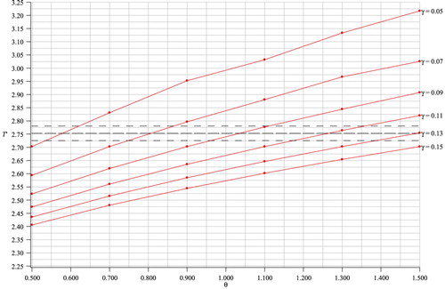
Figure 9. Variation in Euclidean distance for $ϵ=0.05$ (finer scale). The horizontal lines of short dashes show $E\pm 1\mathrm{\%}$ for a steel–epoxyadhesive–steel rod.

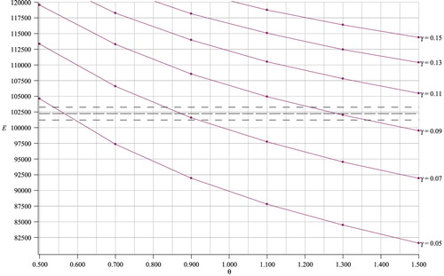
Figure 10. Variation in solotone period for $ϵ=0.05$ (even finer scale).

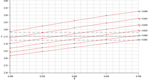
Figure 11. Variation in Euclidean distance for $ϵ=0.05$ (even finer scale).

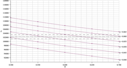
Table 3. Sensitivity of $c_2$ estimates. The values in columns 2 and 3 come from Figures 8 and 9. Figures 10 and 11 were used for columns 6 and 7. Columns 5 and 9 give the relative percentage error for $c_2$.

Variation in $T^{\prime }$ and E	γ	θ	$c_2$	%	γ	θ	$c_2$	%
$T^{\prime }+1\mathrm{\%}$	0.05	0.62	294.5	1.8	0.055	0.678	322.05	7.4
$T^{\prime }-1\mathrm{\%}$	0.05	0.54	256.5	14.5	0.055	0.587	278.83	7.1
$E+1\mathrm{\%}$	0.05	0.54	256.5	14.5	0.055	0.600	285.00	5.0
$E-1\mathrm{\%}$	0.05	0.59	280.3	6.6	0.055	0.665	315.88	5.3

Figure 12. Schematic of a solid composite rod showing a narrow porous region.

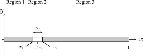
Table 4. Thermal conductivity $k_{1,2}$, specific heat capacity $c_{1,2}$, and relative discontinuities $k_2/k_1$ and $c_2/c_1$ for aluminium and porous aluminium.

Aluminium	Porous Aluminium (4.32%)	RelativeDiscontinuities
$k_1=96.2$	$k_2=87.51$	$\gamma =0.91$
$c_1=963$	$c_2=886.7$	$\theta =0.92$

Figure 13. Solotone period $T^{\prime }$ plotted against the position of the centre of the porous region $x_m$. The porous region is of width $2ϵ$ where $ϵ=0.001$ (asterisk), 0.01 (diamond) and 0.025 (solid circle). The horizontal line of long dashes indicates the solotone period for $x_m=0.2$ and $ϵ=0.01$. The lines of short dashes show $T^{\prime }\pm 5\mathrm{\%}$.

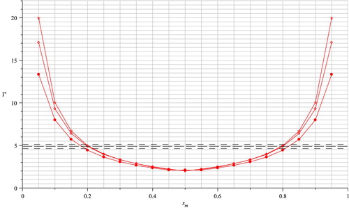
Figure 14. Robin boundary conditions with h = 500. Solotone period $T^{\prime }$ plotted against the position of the porous region $x_m$. The porous region is of width $2ϵ$ where $ϵ=0.001$ (asterisk), 0.01 (diamond) and 0.025 (solid circle). The horizontal line of long dashes indicates the solotone period for $x_m=0.2$ and $ϵ=0.01$. The lines of short dashes show $T^{\prime }\pm 5\mathrm{\%}$.

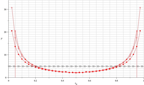
Figure 15. Cross-section of a solid composite sphere with n layers. Each layer possesses a different thermal conductivity $k_i$ and a different thermal diffusivity ${\alpha }_i$.

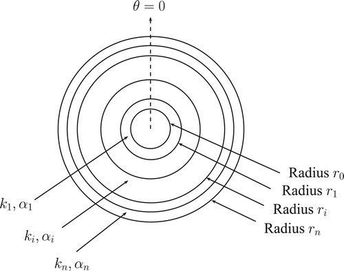
Figure 16. Cross-section of a three-layer solid composite hemisphere. Each layer possesses a different thermal conductivity $k_i$ and a different thermal diffusivity ${\alpha }_i$.

Table 5. Elements of the determinant forming the left-hand side of Equation (7(7) $\left|\begin{array}{cccccc}{C}_{1in}& C_{2in}& 0& 0& 0& 0\\ x_{11}& x_{12}& x_{13}& x_{14}& 0& 0\\ y_{11}& y_{12}& y_{13}& y_{14}& 0& 0\\ 0& 0& x_{21}& x_{22}& x_{23}& x_{24}\\ 0& 0& y_{21}& y_{22}& y_{23}& y_{24}\\ 0& 0& 0& 0& C_{1out}& C_{2out}\end{array}\right|=0.$(7) ).

C	x	y
$C_{1in}=A_{in}{R}_J^{\prime }({\lambda }_{1mp}{r}_0)+B_{in}{R}_J({\lambda }_{1mp}{r}_0)$	$x_{i1}=R_J({\lambda }_{imp}{r}_i)$	$y_{i1}=k_i{R}_J^{\prime }({\lambda }_{imp}{r}_i)$
$C_{2in}=A_{in}{R}_Y^{\prime }({\lambda }_{1mp}{r}_0)+B_{in}{R}_Y({\lambda }_{1mp}{r}_0)$	$x_{i2}=R_Y({\lambda }_{imp}{r}_i)$	$y_{i2}=k_i{R}_Y^{\prime }({\lambda }_{imp}{r}_i)$
$C_{1out}=A_{out}{R}_J^{\prime }({\lambda }_{nmp}{r}_n)+B_{out}{R}_J({\lambda }_{nmp}{r}_n)$	$x_{i3}=-R_J({\lambda }_{i+1,mp}{r}_i)$	$y_{i3}=-k_{i+1}{R}_J^{\prime }({\lambda }_{i+1,mp}{r}_i)$
$C_{2out}=A_{out}{R}_Y^{\prime }({\lambda }_{nmp}{r}_n)+B_{out}{R}_Y({\lambda }_{nmp}{r}_n)$	$x_{i4}=-R_J({\lambda }_{i+1,mp}{r}_i)$	$y_{i4}=-k_{i+1}{R}_Y^{\prime }({\lambda }_{i+1,mp}{r}_i)$

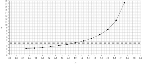
Figure 17. First differences for three values of $r_2/r_0$, namely $r_2/r_0=2.5$ (solid line), $r_2/r_0=4.0$ (dashed line) and $r_2/r_0=5.5$ (dash-dotted line). The corresponding solotone periodicities are 2.07, 3.99 and 17.26.

Figure 18. Three-layer solid composite hemisphere. The objective is to determine the size of the middle hemispherical layer by analysing the solotone effect.

Figure 19. Solotone period $T^{\prime }$ plotted against $\overline{r}$. A solotone period of length 4 is indicated by long dashes. The lines of short dashes show $T^{\prime }\pm 5\mathrm{\%}$.