Analytical solutions for some unsteady flows of fluids with linear dependence of viscosity on the pressure

Figures & data

Figure 1. Illustration of the flow for the boundary value problem under consideration.

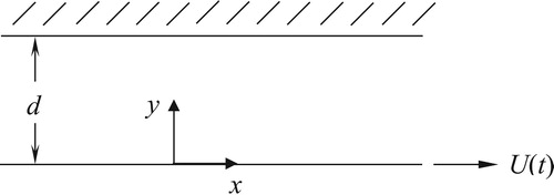
Figure 2. Profiles of steady component $u_{Cp}(y)$ of $u_C(y,t)$ given by equations (42) and (44)₁ for two different values of $\beta$.

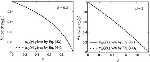
Figure 3. Profiles of the steady-state component $u_{cp}(y,t)$ of $u_c(y,t)$ given by equations (52) and (56) for two different values of $\beta$ and $t=10$.

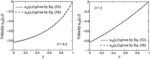
Figure 4. Profiles of the stead-state component $u_{sp}(y,t)$ of $u_s(y,t)$ given by equations (54) and (57) for two different values of $\beta$ and $t=10$.

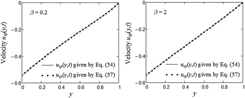
Figure 5. Velocity profiles corresponding to a unit step increase in boundary velocity, given by equation (39), evaluated at three different $\beta$ values at $t=0.1$.

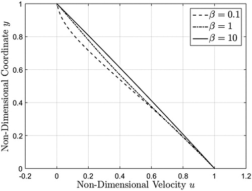
Figure 6. Velocity profiles corresponding to a unit step increase in boundary velocity, given by equation (39), evaluated at three different $\beta$ values at $t=1$.

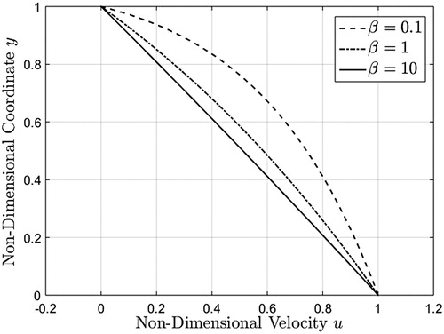
Figure 7. Shear stress profiles corresponding to a unit step increase in boundary velocity, given by equation (40), evaluated at three different $\beta$ values at $t=0.1$.

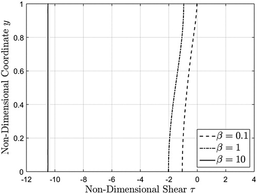
Figure 8. Shear stress profiles corresponding to a unit step increase in boundary velocity, given by equation (40), evaluated at three different $\beta$ values at $t=1$.

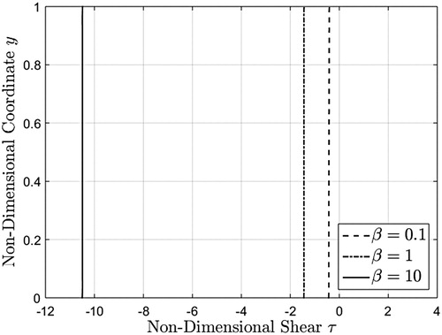
Figure 9. Midplane velocity as a function of time corresponding to a unit step increase in boundary velocity, given by equation (39), evaluated at three different $\beta$ values.

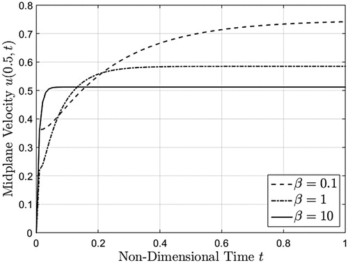
Figure 10. Lower wall shear stress as a function of time corresponding to a unit step increase in boundary velocity, given by equation (40), evaluated at three different $\beta$ values.

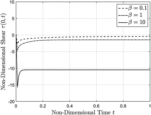
Figure 11. Velocity profiles corresponding to a sinusoidal boundary velocity, given by equations (51)₂, (54) and (55), evaluated at three different $\beta$ values at $\omega t=\pi /2$.

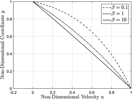
Figure 12. Velocity profiles corresponding to a sinusoidal boundary velocity, given by equations (51)₂, (54) and (55), evaluated at three different $\beta$ values at $\omega t=\pi$.

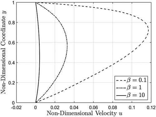
Figure 13. Velocity profiles corresponding to a sinusoidal boundary velocity, given by equations (51)₂, (54) and (55), evaluated at three different $\beta$ values at $\omega t=3\pi /2$.

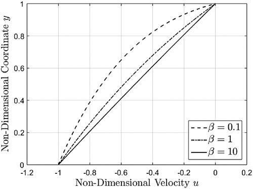
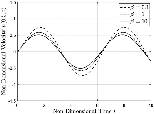
Figure 14. Midplane velocity as a function of time corresponding to a sinusoidal boundary velocity, given by equations (51)₂, (54) and (55), evaluated at three different $\beta$ values.