Spectral graph wavelet regularization and adaptive wavelet for the backward heat conduction problem

Figures & data

Figure 1. The graph arising from regular one-dimensional mesh and its discretization.

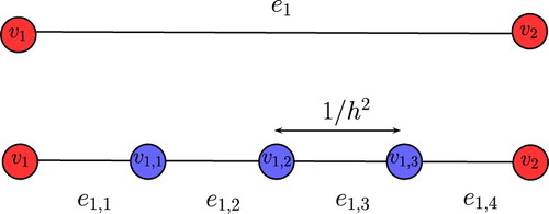
Figure 2. The scaling kernel $\mathsf{\text{h}}(\lambda )$ and wavelet generating kernels $g(t_j(\lambda ))$ for $J=4,{\lambda }_{max}=4.038$: (a) $\mathsf{\text{h}}(\lambda )$ and (b) $g(t_j(\lambda ))$.

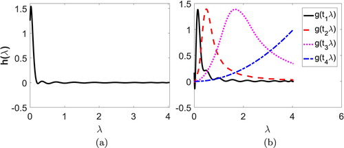
Figure 3. The scaling and wavelet function for J = 4: (a) scaling function, (b) $t_1=9.92$, (c) $t_2=2.89$, (d) $t_3=0.84$, (e) $t_4=0.23$.

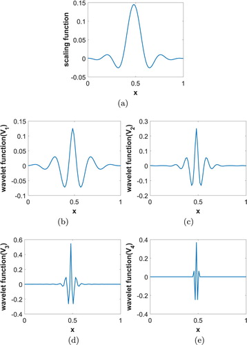
Figure 4. The wavelet kernel $g({\mathrm{t}}_4\lambda )$ and its approximated polynomial $p_4$ using $M_4=20$.

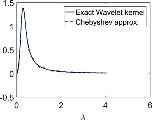
Figure 5. Plot of modified wave number versus wave number.

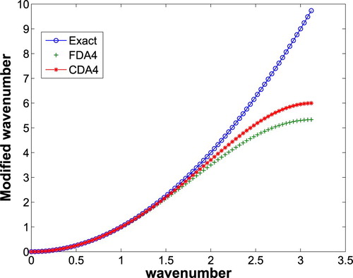
Figure 6. Test function 1 and reconstructed function for (a) $ϵ={10}^{-1}$ and (b) $ϵ={10}^{-4}.$

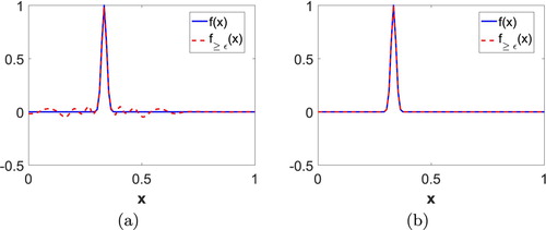
Figure 7. Compression error versus (a) ε and (b) $N(ϵ)$ for test function 1.

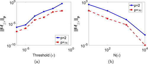
Figure 8. Test function 2 and corresponding reconstructed function for different values of ε: (a) test function 2, (b) $f_{\ge ϵ}$ for $ϵ={10}^{-1}$, (c) $f_{\ge ϵ}$ for $ϵ={10}^{-4}$.

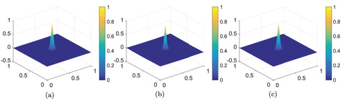
Figure 9. Compression error versus (a) ε and (b) $N(ϵ)$ for test function 2.

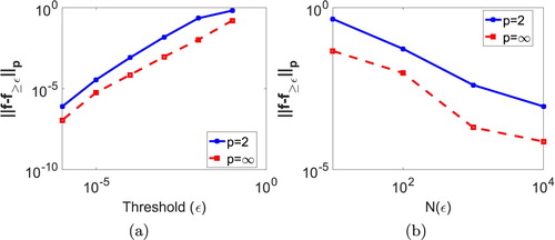
Figure 10. Wavelet coefficients $d_k^j$ at different value of j for two different test functions: (a) $d_k^j$ for test function 1 and (b) $d_k^j$ for sawtooth function with discontinuity at x = 0.5.

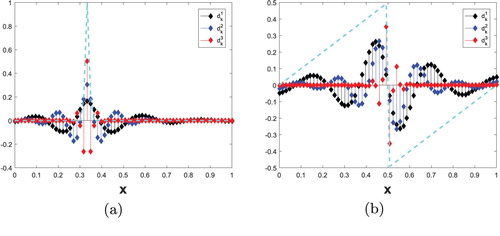
Figure 11. Adaptive node generation for path graph.

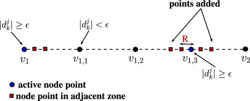
Figure 12. Adaptive node generation for 2-d grid graph.

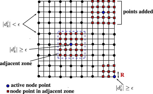
Figure 13. Functions and the corresponding adaptive node arrangements in one-dimensional setting for R = 0.1 and M = 6. (a) Test function 1, (b) Sawtooth function with discontinuity at x = 0.5.

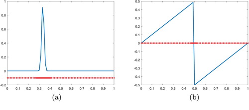
Figure 14. Function and the corresponding adaptive node arrangement in two-dimensional setting for R = 0.1 and M = 6: (a) Test function 2 and (b) adaptive grid.

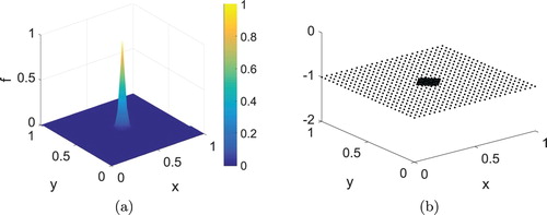
Figure 15. Test function with noise and corresponding regularized data: (a) test function 1 with noise, (b) filtered function, (c) sawtooth function with discontinuity at x = 0.5 with noise and (d) filtered function.

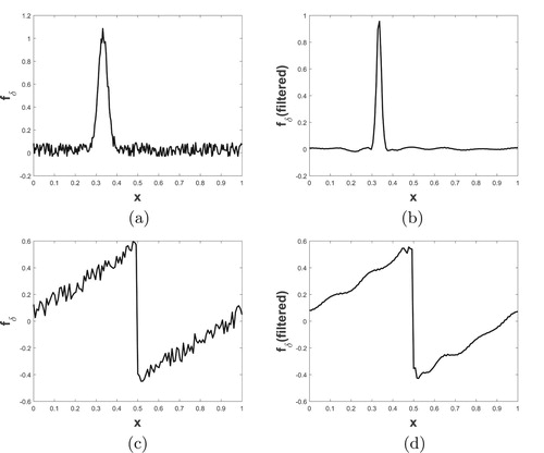
Figure 16. Evolution of the solution and dynamically adapted node arrangement for test problem 1 using $ϵ={10}^{-3},R=0.1,M=6$: (a) $T=0.1(N(ϵ)=176)$, (b) $T=0.4(N(ϵ)=248)$, (c) $T=0.8(N(ϵ)=301)$, (d) $T=1(N(ϵ)=377)$.

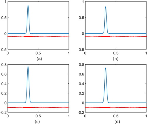
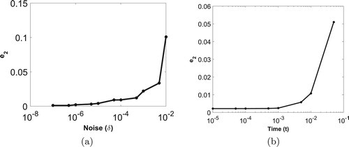
Figure 17. Plot of (a) error versus noise parameter δ with fixed $T={10}^{-2}$ and (b) error versus time T with fixed $\delta ={10}^{-3}$ for test problem 1.

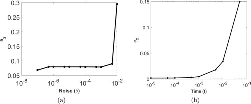
Figure 18. Plot of error versus $N(ϵ)$ for test problem 1.

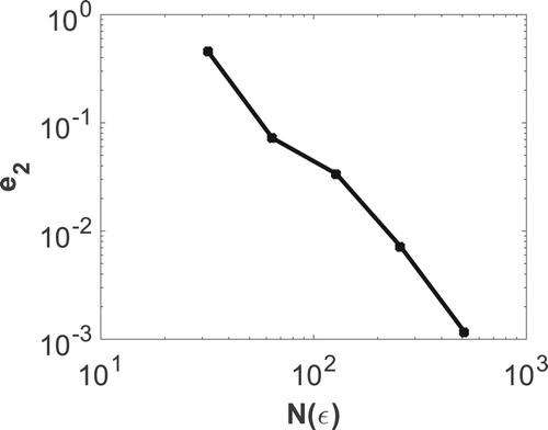
Table 1. Comparison of relative error for test problem 1 between Fu et al. [15] and ASGWM.

Time (T)	$e_2$ (Fu et al.)	$e_2$ (ASGWM)	CPU (Fu et al.)	CPU (ASGWM)
0.01	$6.24\times {10}^{-3}$	$8.47\times {10}^{-3}$	0.93	0.76
0.1	$1.21\times {10}^{-2}$	$0.82\times {10}^{-2}$	2.43	0.91
0.5	$7.53\times {10}^{-2}$	$7.07\times {10}^{-2}$	3.81	1.64
1	$2.60\times {10}^{-1}$	$3.19\times {10}^{-1}$	5.30	2.97

Figure 19. (a) Θ versus ε for test problem 1 at $t={10}^{-2}$. (b) $e_2$ versus ε for test problem 1.

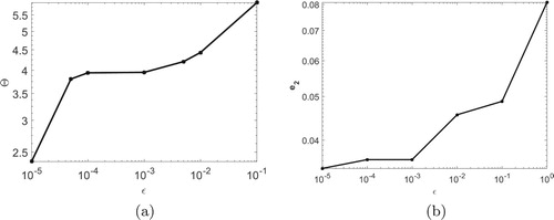
Figure 20. Evolution of the regularized numerical solution and corresponding dynamically adapted node arrangement for test problem 2 using $ϵ={10}^{-3},R=0.1,M=6$. (a) Solution for T = 0.1. (b) Adaptive node arrangement ($N(ϵ)=1258$). (c) Solution for T = 0.2. (d) Adaptive node arrangement ($N(ϵ)=2665$). (e) Solution for T = 0.4. (f) Adaptive node arrangement ($N(ϵ)=4382$). (g) Solution for T = 0.8. (h) Adaptive node arrangement ($N(ϵ)=4724$).

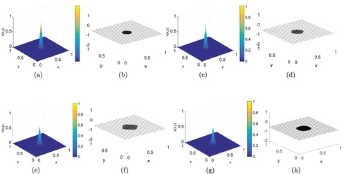
Table 2. The performance of ASGWM for test problem 2 with regularization.

ε	${10}^{-1}$	${10}^{-2}$	${10}^{-3}$	${10}^{-4}$	${10}^{-5}$
$\mathrm{CPU}(ϵ)$	0.51	0.68	0.73	0.891	1.21
Θ	6.078	4.55	4.24	3.479	2.561

Figure 21. Plot of (a) error versus noise parameter δ with fixed $T={10}^{-2}$ and (b) error versus time T with fixed $\delta ={10}^{-3}$ for test problem 2.

Fu CL, Xiong XT, Qian Z. Fourier regularization for a backward heat equation. J Math Anal Appl. 2007;331:472–480. doi: 10.1016/j.jmaa.2006.08.040

 Google Scholar