An inverse problem of a simultaneous reconstruction of the dielectric constant and conductivity from experimental backscattering data

Figures & data

Figure 1. A schematic diagram illustrating our experimental configuration. The transmitter is the antenna put in front of the detector placing the far-field measurement site. The backscattering waves hit the antenna before reaching the detectors. This causes a certain noise in the data.

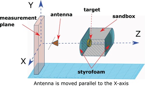
Figure 2. Aluminium cylinder; see Tables 1–2 for further details. (a) and (b) A clear advantage of the data propagation procedure in data preprocessing. (a) Real part of raw and propagated data at $\alpha =0.4$. (b) Imaginary part of raw and propagated data at $\alpha =0.4$. (c) Left: Aluminium cylinder (cf. [2]). Middle: Image of computed dielectric constant. Right: Image of computed conductivity.

Table 1. Chosen wavenumbers, frequencies and wavelength for Examples 1–5.

Example	1	2	3	4	5
k	8.51	6.62	11.43	9.55	8.79
Frequency (GHz)	4.06	3.16	5.45	4.55	4.19
Wavelength (cm)	7.39	9.49	5.50	6.59	7.16

Table 2. True $c_{\mathrm{true}}$, computed $max(c_{\mathrm{comp}})$ dielectric constants and computed conductivity $max({\sigma }_{\mathrm{comp}})$ of Examples 1–5 of experimental data. True values of dielectric constants were taken from: (a) Examples 1, 4, 5: formula (7.2) of [40], (b) Example 2 (clear water) [38], (c) Example 3 [41].

Example	1	2	3	4	5
Object	Metallic cylinder	Water	Wood	Metallic letter ‘A’	Metallic letter ‘O’
$max(c_{\mathrm{comp}})$	28.78	23.18	6.33	16.24	16.22
$c_{\mathrm{true}}$	$[10,30]$	23.8	$[2,6]$	$[10,30]$	$[10,30]$
$max({\sigma }_{\mathrm{comp}})$	2.33	0.94	0.94	1.32	1.66

Figure 3. A bottle of clear water; see Tables 1–2 for further details. Note that we can image even a tiny part of it: the cap of this bottle, at least when we compute the dielectric constant. (a) and (b) A serious data improvement due to the data propagation procedure. (a) Real part of raw and propagated data at $\alpha =0.4$. (b) Imaginary part of raw and propagated data at $\alpha =0.4$. (c) Left: Glass bottle (cf. [2]). Middle: Image of computed dielectric constant. Right: Image of computed conductivity.

Figure 4. U-shaped piece of dry wood; see Tables 1–2 for further details. Note that we can image even the void of this nonconvex target. It is well known that imaging of nonconvex targets with voids in them is a quite challenging goal. This is especially true for the most challenging case we consider: backscattering nonoverdetermined data. (a) Real part of raw and propagated data at $\alpha =0.5$. (b) Imaginary part of raw and propagated data at $\alpha =0.5$. (c) Left: U-shaped piece of dry wood (cf. [2]). Middle: Image of computed dielectric constant. Right: Image of computed conductivity.

Figure 5. A-shaped metallic target. The same comments as ones for Figure 4 are applicable here. (a) Real part of raw and propagated data at $\alpha =0.2$. (b) Imaginary part of raw and propagated data at $\alpha =0.2$. (c) Left: Metallic letter ‘A’ (cf. [2]). Middle: Image of computed dielectric constant. Right: Image of computed conductivity.

Figure 6. O-shaped metallic target. The same comments as ones for Figure 4 are applicable here. (a) Real part of raw and propagated data at $\alpha =0.6$. (b) Imaginary part of raw and propagated data at $\alpha =0.6$. (c) Left: Metallic letter ‘O’ (cf. [2]). Middle: Image of computed dielectric constant. Right: Image of computed conductivity.

Khoa VA, Bidney GW, Klibanov MV, et al. Convexification and experimental data for a 3D inverse scattering problem with the moving point source. Inverse Probl. 2020. doi:10.1088/1361-6420/ab95aa.

 Google Scholar

Kuzhuget AV, Beilina L, Klibanov MV, et al. Blind backscattering experimental data collected in the field and an approximately globally convergent inverse algorithm. Inverse Probl. 2012;28:095007.

 Google Scholar

Thành NT, Beilina L, Klibanov MV, et al. Imaging of buried objects from experimental backscattering time-dependent measurements using a globally convergent inverse algorithm. SIAM J Imaging Sci. 2015;8(1):757–786.

 Google Scholar

Clipper Controls Inc. (n.d.) Dielectric constants of various materials. http://www.clippercontrols.com/pages/Dielectric-Constant-Values.html#W.

 Google Scholar